Basic material science energy calculation
Note
Cost of compute (💵) ~ $0.17 This is roughly how much it will cost you to try out this tutorial in covalent cloud using the same compute resources.
In this tutorial we will see how to calculate energy of a list of materials using covalent cloud in parallel, we will be spinning up almost 360 cores of compute to do this calculation (which we will see happens in order of minutes !).
First lets write the code to calculate the energy of a single material, then we will parallelize it. We will be using ase to create the structure and gpaw to calculate the energy.
1. Install PAW data sets
We will first write a function to download the PAW data sets. Because covalent cloud provides easy abstractions for persistent volumes, we can download the data sets once and use them across multiple experiments. We will store them in /volumes/chem_data/
from pathlib import Path
import requests
import tarfile
import os

def download_and_install_paw_datasets(setup_base_path='/volumes/chem_data/',version = "0.9.20000"):
    paw_url = f'https://wiki.fysik.dtu.dk/gpaw-files/gpaw-setups-{version}.tar.gz'
    setup_base_path = Path(setup_base_path)
    setup_path = setup_base_path / f'gpaw-setups-{version}'

    # Check if the setup directory and its contents already exist
    if setup_path.exists() and any(setup_path.iterdir()):
        print(f"PAW datasets already installed at: {setup_path}")
        return str(setup_path)

    setup_base_path.mkdir(parents=True, exist_ok=True)  # Ensure base path exists
    tar_path = setup_base_path / f'gpaw-setups-{version}.tar.gz'

    # Download and extract PAW datasets
    with open(tar_path, 'wb') as file:
        file.write(requests.get(paw_url).content)
    with tarfile.open(tar_path, 'r:gz') as tar:
        tar.extractall(path=setup_base_path)

    print(f"PAW datasets installed at: {setup_path}")

    return str(setup_path)
2. Calculate energy of a single material
We do a simple DFT calculation to calculate the energy of the system and return the energy
def get_energy(system, calc_kwargs={}):
    from gpaw import GPAW
    from gpaw import setup_paths

    #will be downloaded only once as we are using the persistant volume mounted at /volumes/chem_data/
    path=download_and_install_paw_datasets(setup_base_path='/volumes/chem_data/')
    setup_paths.insert(0, path)

    default_calc_kwargs = {
        'xc': 'PBE',
        'mode': 'PW'
    }

    calc_kwargs = {**default_calc_kwargs, **calc_kwargs}

    calc = GPAW(**calc_kwargs)
    system.set_calculator(calc)
    return system.get_potential_energy()
3. Covalent Cloud setup
3.1. To setup your covalent cloud, lets import the cloud packages and save the API Key that you can find on the dashboard. If you don't have an account, you can sign up here
import covalent_cloud as cc
import covalent as ct

API_KEY=<your_API_KEY_as_string> #replace with your API key

cc.save_api_key(API_KEY)
3.2. We create the required environment, for more details on how to create an environment, refer to the documentation
cc.create_env(
    name="dft_new",pip= ["ase"],
    conda={"channels": ["conda-forge"],
          "dependencies": ["blas","cupy","openmpi",
                          "openssh","scalapack","fftw",
                          "gpaw"]})
Environment Already Exists.
3.3. We now create a low compute executor for running auxiliary tasks.
We then attach this executor to a lattice which defines our workflow, to accept a list of systems and a high compute executor to run the DFT calculations in parallel. Note that our workflow is defined by @ct.lattce decorator which defines the depedencies between electron functions.
#lets define a low compute executor
low_compute = cc.CloudExecutor(env="dft_new", num_cpus=2, memory="1GB",
                               time_limit="1 hours")
@ct.lattice(executor=low_compute, workflow_executor=low_compute)
def calculate_energy(systems,executor,calculator_kwargs={}):
    # Let us make it accept a single system or a list of systems
    if type(systems) is not list:
        systems = [systems]

    result=[]

    #Let us convert the get_energy function to a cloud electron function
    # with @ct.electron decorator and attach the executor to it
    get_energy_electron=ct.electron(get_energy,executor=executor)

    #loop over systems and calculate the energy as you would normally do
    for system in systems:
        result.append(get_energy_electron(system,calculator_kwargs))
    return result
3.4 After this we create the persistent volume to store and access the PAW data sets and finally create a dispatch the workflow using cc.dispatch with required inputs.
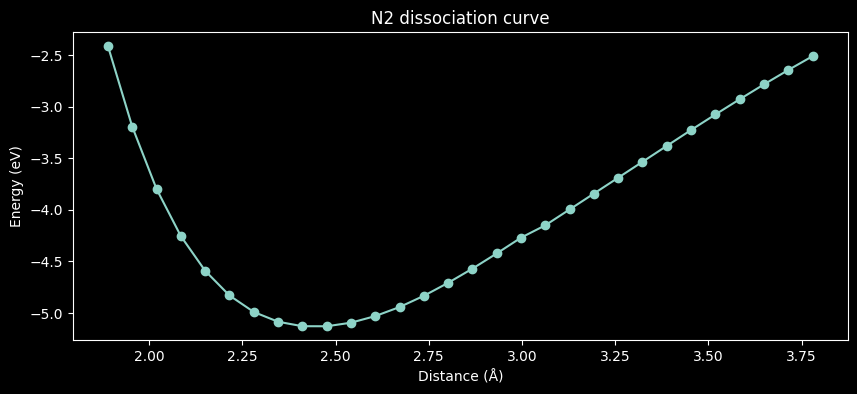
For this example, we are creating a list of Nitrogen molecules at various bond lengths and calculating the energy of each molecule.
import numpy as np
from ase import Atoms

n_steps=30
molecules = [Atoms('2N', [(0., 0., 0.), (0., 0., d)])
            for d in np.linspace(1.0, 2.0, n_steps)]
for molecule in molecules:
    molecule.center(vacuum=5)
We define the high compute resource using num_cpus=12 here, which means we will be using 12 cores to calculate the energy of each molecule.
high_compute = cc.CloudExecutor(env="dft_new",
                                num_cpus=12,
                                memory="1GB",
                                time_limit="1 hours")
We create the volume and attach it to the environment, so that the PAW data sets are available to the DFT calculations.
Finally we dispatch the workflow with the list of systems and the high compute resource. We get back the dispatch ID which we can later use whenever we want to query back the result and metadata associated with the result.
calculation_parameters = {"xc": "PBE", "mode": "lcao"}

volume=cc.volume("/chem_data")


calc_id=cc.dispatch(calculate_energy,volume=volume)(systems=molecules,
                                                    executor= high_compute,
                                                    calculator_kwargs=calculation_parameters)
print("Calculation ID: ",calc_id)
Output()
Calculation ID: 50226d36-b8ca-45bf-b204-765835bfabb6
You should now see a new dispatch appear on the dispatch page of the UI at https://app.covalent.xyz/dispatches
calc_result=cc.get_result(calc_id,wait=True)

time_taken=(calc_result.end_time-calc_result.start_time).total_seconds()
print(f"Total time taken for scaling up {12*n_steps} cores : {time_taken / 60:.3} minutes")
Total time taken for scaling up 360 cores : 4.5 minutes
Note
As seen the total calculation takes around 4.5 minutes of wall time to calculate the energy of 30 systems. This includes the spin up time of the compute resources along with the movement of the environment images to the compute resources and the actual calculation time.
We load the result as all the heavy part of result objects are always lazy loaded
calc_result.result.load()

import matplotlib.pyplot as plt
from ase.units import Bohr

energies = [energy / len(molecule) for energy, molecule in zip(calc_result.result.value, molecules)]
distances = [molecule.get_distance(0, 1) / Bohr for molecule in molecules]

fig, ax = plt.subplots(figsize=(10, 4))
ax.plot(distances, energies, 'o-')
ax.set(title='N2 dissociation curve', xlabel='Distance (Å)', ylabel='Energy (eV)')
plt.show()
Full Code
from pathlib import Path
import requests
import tarfile
import os
import covalent_cloud as cc
import covalent as ct
import numpy as np
from ase import Atoms

# Install PAW data sets
def download_and_install_paw_datasets(setup_base_path='/volumes/chem_data/',version = "0.9.20000"):
    paw_url = f'https://wiki.fysik.dtu.dk/gpaw-files/gpaw-setups-{version}.tar.gz'
    setup_base_path = Path(setup_base_path)
    setup_path = setup_base_path / f'gpaw-setups-{version}'

    # Check if the setup directory and its contents already exist
    if setup_path.exists() and any(setup_path.iterdir()):
        print(f"PAW datasets already installed at: {setup_path}")
        return str(setup_path)

    setup_base_path.mkdir(parents=True, exist_ok=True)  # Ensure base path exists
    tar_path = setup_base_path / f'gpaw-setups-{version}.tar.gz'

    # Download and extract PAW datasets
    with open(tar_path, 'wb') as file:
        file.write(requests.get(paw_url).content)
    with tarfile.open(tar_path, 'r:gz') as tar:
        tar.extractall(path=setup_base_path)

    print(f"PAW datasets installed at: {setup_path}")

    return str(setup_path)

# Calculate energy of a single material
def get_energy(system, calc_kwargs={}):
    from gpaw import GPAW
    from gpaw import setup_paths

    #will be downloaded only once as we are using the persistant volume mounted at /volumes/chem_data/
    path=download_and_install_paw_datasets(setup_base_path='/volumes/chem_data/')
    setup_paths.insert(0, path)

    default_calc_kwargs = {
        'xc': 'PBE',
        'mode': 'PW'
    }

    calc_kwargs = {**default_calc_kwargs, **calc_kwargs}

    calc = GPAW(**calc_kwargs)
    system.set_calculator(calc)
    return system.get_potential_energy()

# Covalent Cloud setup
API_KEY=<your_API_KEY_as_string> #replace with your API key

cc.save_api_key(API_KEY)

cc.create_env(
    name="dft_new",pip= ["ase"],
    conda={"channels": ["conda-forge"],
          "dependencies": ["blas","cupy","openmpi",
                          "openssh","scalapack","fftw",
                          "gpaw"]})

#lets define a low compute executor
low_compute = cc.CloudExecutor(env="dft_new", num_cpus=2, memory="1GB",
                               time_limit="1 hours")

@ct.lattice(executor=low_compute, workflow_executor=low_compute)
def calculate_energy(systems,executor,calculator_kwargs={}):
    # Let us make it accept a single system or a list of systems
    if type(systems) is not list:
        systems = [systems]

    result=[]

    #Let us convert the get_energy function to a cloud electron function
    # with @ct.electron decorator and attach the executor to it
    get_energy_electron=ct.electron(get_energy,executor=executor)

    #loop over systems and calculate the energy as you would normally do
    for system in systems:
        result.append(get_energy_electron(system,calculator_kwargs))
    return result

n_steps=30
molecules = [Atoms('2N', [(0., 0., 0.), (0., 0., d)])
            for d in np.linspace(1.0, 2.0, n_steps)]
for molecule in molecules:
    molecule.center(vacuum=5)

high_compute = cc.CloudExecutor(env="dft_new",
                                num_cpus=12,
                                memory="1GB",
                                time_limit="1 hours")

calculation_parameters = {"xc": "PBE", "mode": "lcao"}

volume=cc.volume("/chem_data")


calc_id=cc.dispatch(calculate_energy,volume=volume)(systems=molecules,
                                                    executor= high_compute,
                                                    calculator_kwargs=calculation_parameters)
print("Calculation ID: ",calc_id)


calc_result=cc.get_result(calc_id,wait=True)

time_taken=(calc_result.end_time-calc_result.start_time).total_seconds()
print(f"Total time taken for scaling up {12*n_steps} cores : {time_taken / 60:.3} minutes")

calc_result.result.load()

import matplotlib.pyplot as plt
from ase.units import Bohr

energies = [energy / len(molecule) for energy, molecule in zip(calc_result.result.value, molecules)]
distances = [molecule.get_distance(0, 1) / Bohr for molecule in molecules]

fig, ax = plt.subplots(figsize=(10, 4))
ax.plot(distances, energies, 'o-')
ax.set(title='N2 dissociation curve', xlabel='Distance (Å)', ylabel='Energy (eV)')
plt.show()
Thats it ! We have calculated the energy of a list of materials in parallel using covalent cloud. We have used the following parts of covalent cloud in this tutorial: