FashionMNIST tutorial

Fashion-MNIST is a dataset of Zalando's article images, featuring a training set containing 60,000 instances and a test set of 10,000 examples. Each image measures 28 pixels in both height and width for a total of 784 pixels. Every pixel is assigned a single value from 0 to 255 that represents its lightness or darkness, with higher values indicating darker shades. Both the training and test datasets consist of 785 columns.

In this tutorial, we use Covalent to train a Neural Network (NN) using PyTorch. All the computations will be executed on Covalent Cloud for the total cost of ~$0.25.

As written, this tutorial requires a local environment with the following packages.

covalent-cloud>=0.81.0
pandas==2.2.3
plotly==5.18.0
torch==2.4.1
torchvision==0.19.1

Getting started

Start by importing the required packages.

import covalent as ct
import covalent_cloud as cc
import plotly.express as px
import torch
import torch.nn as nn
import torch.optim as optim
from torch.utils.data import DataLoader
from torchvision.datasets import FashionMNIST
from torchvision.transforms import ToTensor

Cloud environment

Create a Covalent Cloud environment for remote code execution.

cc.save_api_key("YOUR-API-KEY")  # NOTE: Paste your actual API key here
cc.create_env(
    name="fashionmnist",
    pip=[
        "torch==2.4.1",
        "torchvision==0.19.1",
        "numpy==1.23.5",
        "plotly==5.18.0",
        "pandas==2.2.3",
    ],
    wait=True
)

Cloud storage

Let's also create a cloud storage volume to store trained models.

volume = cc.volume("/models")

Compute resources

Executors specify compute resources together with a cloud environment.

Here we use one executor for CPU-only tasks and another for GPU tasks.

cpu_executor = cc.CloudExecutor(
    env="fashionmnist",
    num_cpus=2,
    memory="8GB",
    time_limit="01:00:00",  # 1 hour
)

gpu_executor = cc.CloudExecutor(
    env="fashionmnist",
    num_cpus=2,
    memory="8GB",
    num_gpus=1,
    gpu_type="l40",
    time_limit="02:00:00",  # 2 hours
)

Covalent tasks for training the classifier

Here we will build a classifier for the FashionMNIST dataset using a simple neural network.

class SimpleNN(nn.Module):
    def __init__(self):
        super(SimpleNN, self).__init__()
        self.fc1 = nn.Linear(28 * 28, 128)
        self.relu = nn.ReLU()
        self.fc2 = nn.Linear(128, 10)

    def forward(self, x):
        x = x.view(-1, 28 * 28)
        x = self.fc1(x)
        x = self.relu(x)
        x = self.fc2(x)
        return x

We define a data loader task to load and transform data.

@ct.electron(executor=cpu_executor)
def data_loader(
    batch_size: int,
    train: bool,
    download: bool = True,
    data_dir: str = "./data",
    shuffle: bool = True,
):
    """Initialize a data loader for the FashionMNIST dataset."""
    data = FashionMNIST(
        root=data_dir, train=train, download=download, transform=ToTensor()
    )
    return DataLoader(data, batch_size=batch_size, shuffle=shuffle)

This next task does the actual model training using a standard optimizer.

@ct.electron(executor=gpu_executor)
def train_model(dataloader, num_epochs: int, learning_rate: float):
    """Train the simple neural network model."""

    model = SimpleNN().to("cuda")
    criterion = nn.CrossEntropyLoss().to("cuda")
    optimizer = optim.Adam(model.parameters(), lr=learning_rate)

    losses = []
    # Training the model
    for epoch in range(num_epochs):
        model.train()
        running_loss = 0.0

        for inputs, labels in dataloader:
            inputs, labels = inputs.to("cuda"), labels.to("cuda")

            optimizer.zero_grad()

            outputs = model(inputs).to("cuda")
            loss = criterion(outputs, labels)
            loss.backward()

            optimizer.step()
            running_loss += loss.item()
        print(
            f"{epoch+1}/{num_epochs}: loss {running_loss/len(dataloader)}"
        )
        losses.append(running_loss / len(dataloader))

    # save model to volume
    model_file_path = volume / "model.pth"
    torch.save(model.state_dict(), model_file_path)
    return model_file_path, losses

We define the following task to evaluate the model after training.

@ct.electron(executor=gpu_executor)
def test_model(dataloader, model_file_path):
    """Test the trained neural network model."""
    model = SimpleNN()
    model.load_state_dict(torch.load(model_file_path))

    model = model.to("cuda")
    model.eval()

    correct = 0
    total = 0
    with torch.no_grad():
        for inputs, labels in dataloader:
            inputs, labels = inputs.to("cuda"), labels.to("cuda")

            outputs = model(inputs)

            _, predicted = torch.max(outputs.data, 1)

            total += labels.size(0)
            correct += (predicted == labels).sum().item()

    accuracy = correct / total
    print(f"Accuracy on the test set: {accuracy:.4f}")
    return accuracy

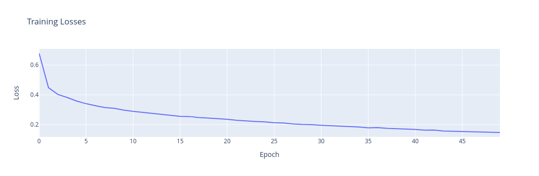
Finally, this task plots the training loss over epochs.

@ct.electron(executor=cpu_executor)
def plot_losses(losses):
    return px.line(
        y=losses, title="Training Losses", labels={"y": "Loss", "x": "Epoch"}
    )

Workflow

Time to put everything together! This is our "main" function inside which we call our electron functions. Unlike tasks (@ct.electron), this function is decorated with @ct.lattice.

@ct.lattice(workflow_executor=cpu_executor, executor=cpu_executor)
def fashionmnist_workflow(train_batch_size: int, test_batch_size: int, epoch_num: int = 5):
    """
    Covalent Cloud workflow that trains a tests a simple neural network
    on the FashionMNIST dataset.
    """
    train_loader = data_loader(train_batch_size, train=True)
    test_loader = data_loader(test_batch_size, train=False, shuffle=False)

    model_path, losses = train_model(
        dataloader=train_loader,
        num_epochs=epoch_num,
        learning_rate=0.001
    )
    accuracy = test_model(
        dataloader=test_loader,
        model_file_path=model_path
    )

    fig = plot_losses(losses)

    return accuracy, fig

Running the workflow

To run the workflow in Covalent Cloud, wrap the lattice function in cc.dispatch then call it with the desired parameters. This returns a unique dispatch ID for querying the results.

dispatch_id = cc.dispatch(fashionmnist_workflow, volume=volume)(
    train_batch_size=256, test_batch_size=64, epoch_num=50
)

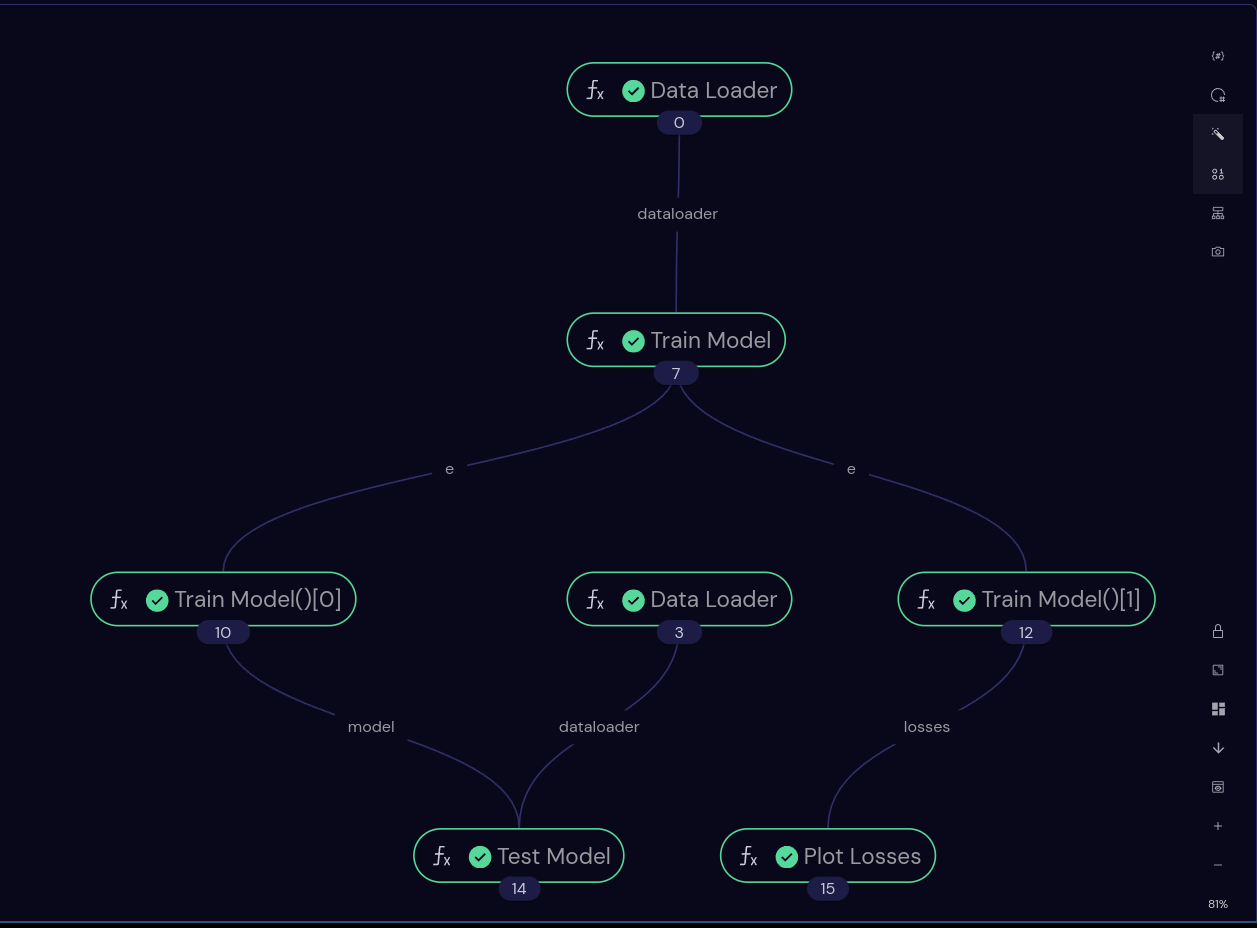
Once the workflow is complete, the transport graph in the Covalent Cloud UI should look something like this:

Results can be retrieved at any time after completion, provided you have the dispatch ID.

accuracy, fig = cc.get_result(dispatch_id).result.load()

Opening the fig object should render a plotly plot of the training loss.

Conclusion

In this tutorial, we created and ran a FashionMNIST classifier. Using Covalent Cloud, we benefitted from a simple and intuitive way to experiment with various hyperparameters, transition between CPU and GPU devices, and save our trained models - all from inside a single Jupyter Notebook.

The full code can be found below.

Full Code

import covalent as ct
import covalent_cloud as cc
import plotly.express as px
import torch
import torch.nn as nn
import torch.optim as optim
from torch.utils.data import DataLoader
from torchvision.datasets import FashionMNIST
from torchvision.transforms import ToTensor

cc.save_api_key("YOUR-API-KEY")  # NOTE: Paste your actual API key here
cc.create_env(
    name="fashionmnist",
    pip=[
        "torch==2.4.1",
        "torchvision==0.19.1",
        "numpy==1.23.5",
        "plotly==5.18.0",
        "pandas==2.2.3",
    ],
    wait=True
)

volume = cc.volume("/models")

cpu_executor = cc.CloudExecutor(
    env="fashionmnist",
    num_cpus=2,
    memory="8GB",
    time_limit="01:00:00",  # 1 hour
)

gpu_executor = cc.CloudExecutor(
    env="fashionmnist",
    num_cpus=2,
    memory="8GB",
    num_gpus=1,
    gpu_type="l40",
    time_limit="02:00:00",  # 2 hours
)


class SimpleNN(nn.Module):
    def __init__(self):
        super(SimpleNN, self).__init__()
        self.fc1 = nn.Linear(28 * 28, 128)
        self.relu = nn.ReLU()
        self.fc2 = nn.Linear(128, 10)

    def forward(self, x):
        x = x.view(-1, 28 * 28)
        x = self.fc1(x)
        x = self.relu(x)
        x = self.fc2(x)
        return x


@ct.electron(executor=cpu_executor)
def data_loader(
    batch_size: int,
    train: bool,
    download: bool = True,
    data_dir: str = "./data",
    shuffle: bool = True,
):
    """Initialize a data loader for the FashionMNIST dataset."""
    data = FashionMNIST(
        root=data_dir, train=train, download=download, transform=ToTensor()
    )
    return DataLoader(data, batch_size=batch_size, shuffle=shuffle)


@ct.electron(executor=gpu_executor)
def train_model(dataloader, num_epochs: int, learning_rate: float):
    """Train the simple neural network model."""

    model = SimpleNN().to("cuda")
    criterion = nn.CrossEntropyLoss().to("cuda")
    optimizer = optim.Adam(model.parameters(), lr=learning_rate)

    losses = []
    # Training the model
    for epoch in range(num_epochs):
        model.train()
        running_loss = 0.0

        for inputs, labels in dataloader:
            inputs, labels = inputs.to("cuda"), labels.to("cuda")

            optimizer.zero_grad()

            outputs = model(inputs).to("cuda")
            loss = criterion(outputs, labels)
            loss.backward()

            optimizer.step()
            running_loss += loss.item()
        print(
            f"{epoch+1}/{num_epochs}: loss {running_loss/len(dataloader)}"
        )
        losses.append(running_loss / len(dataloader))

    # save model to volume
    model_file_path = volume / "model.pth"
    torch.save(model.state_dict(), model_file_path)
    return model_file_path, losses


@ct.electron(executor=gpu_executor)
def test_model(dataloader, model_file_path):
    """Test the trained neural network model."""
    model = SimpleNN()
    model.load_state_dict(torch.load(model_file_path))

    model = model.to("cuda")
    model.eval()

    correct = 0
    total = 0
    with torch.no_grad():
        for inputs, labels in dataloader:
            inputs, labels = inputs.to("cuda"), labels.to("cuda")

            outputs = model(inputs)

            _, predicted = torch.max(outputs.data, 1)

            total += labels.size(0)
            correct += (predicted == labels).sum().item()

    accuracy = correct / total
    print(f"Accuracy on the test set: {accuracy:.4f}")
    return accuracy


@ct.electron(executor=cpu_executor)
def plot_losses(losses):
    """Plot the training losses."""
    return px.line(
        y=losses, title="Training Losses", labels={"y": "Loss", "x": "Epoch"}
    )


@ct.lattice(workflow_executor=cpu_executor, executor=cpu_executor)
def fashionmnist_workflow(train_batch_size: int, test_batch_size: int, epoch_num: int = 5):
    """
    Covalent Cloud workflow that trains a tests a simple neural network
    on the FashionMNIST dataset.
    """
    train_loader = data_loader(train_batch_size, train=True)
    test_loader = data_loader(test_batch_size, train=False, shuffle=False)

    model_path, losses = train_model(
        dataloader=train_loader,
        num_epochs=epoch_num,
        learning_rate=0.001
    )
    accuracy = test_model(
        dataloader=test_loader,
        model_file_path=model_path
    )

    fig = plot_losses(losses)

    return accuracy, fig

if __name__ == "__main__":
    dispatch_id = cc.dispatch(fashionmnist_workflow, volume=volume)(
        train_batch_size=256, test_batch_size=64, epoch_num=50
    )

    accuracy, fig = cc.get_result(dispatch_id, wait=True).result.load()

    print("Accuracy:", accuracy)

We have used the following parts of covalent cloud in this tutorial:

• Persistent volumes
• High compute resources