Scaling Hybrid Quantum Neural Networks across GPUs with Covalent Cloud and CUDA Quantum

In this tutorial, we’ll use Covalent Cloud to access high-power GPUs to simulate quantum circuits with CUDA Quantum. Specifically, we’ll create a hybrid neural network consisting of quantum and classical layers, then train and evaluate using CUDA Quantum and PyTorch.

Covalent Environment

To set up our local environment, pip-install the following packages:

covalent-cloud>=0.81.0
matplotlib==3.9.2
numpy==1.23.5
pillow==11.0.0
torch==2.4.1
torchvision==0.19.1

We also create a Covalent Cloud environment that mirrors some of these local dependencies.

import covalent as ct
import covalent_cloud as cc

cc.save_api_key("YOUR-API-KEY")
cc.create_env(
    name="cuda-quantum",
    pip=[
        "cuda-quantum==0.8.0",  # install in cloud env only
        "matplotlib==3.9.1",
        "torch==2.4.1",
        "torchvision==0.19.1",
    ],
    wait=True
)

Next, we define two Covalent Cloud executors: a CPU-only executor and a GPU-equipped executor. We’ll use the latter for compute-heavy tasks, such as training the neural network. The CPU executor will handle lighter tasks, like downloading data and plotting results.

cpu_executor = cc.CloudExecutor(
    env="cuda-quantum",
    num_cpus=4,
    memory="16GB",
    time_limit=60*60  # 1 hour
)
gpu_executor = cc.CloudExecutor(
    env="cuda-quantum",
    num_gpus=1,
    gpu_type="h100",
    num_cpus=4,
    memory="16GB",
    time_limit=60*60
)

Let’s also create a Covalent Cloud volume named “cudaq” for persistent storage. We will include this volume during dispatch to make it accessible to every task.

volume = cc.volume(VOLUME_NAME)

Hybrid Quantum Neural Network

import matplotlib.pyplot as plt
import numpy as np
import torch
import torch.nn as nn
import torch.nn.functional as F
import torch.optim as optim
from PIL import Image
from torch.autograd import Function
from torchvision import datasets, transforms

Our hybrid neural network will be a simple one, for the sake of example. It consists of a convolutional neural network and an appended quantum layer. The code below is based on this CUDA Quantum tutorial example.

class QuantumFunction(Function):

    def __init__(self, qubit_count: int, device, kernel, thetas):
        """Define the quantum circuit in CUDA Quantum"""
        self.kernel = kernel
        self.theta = thetas
        self.device = device
        qubits = kernel.qalloc(qubit_count)
        self.kernel.h(qubits)
        # Variational gate parameters which are optimised during training.
        kernel.ry(thetas[0], qubits[0])
        kernel.rx(thetas[1], qubits[0])

    def run(self, thetas: torch.tensor) -> torch.tensor:
        """Execute the quantum circuit to output an expectation value"""
        import cudaq  # importing here avoids local package requirement

        exp_ = cudaq.observe(self.kernel, cudaq.spin.z(0), thetas.tolist()).expectation()
        expectation = torch.tensor(exp_, device=self.device)
        return expectation

    @staticmethod
    def forward(ctx, thetas: torch.tensor, quantum_circuit, shift) -> torch.tensor:

        # Save shift and quantum_circuit in context to use in backward.
        ctx.shift = shift
        ctx.quantum_circuit = quantum_circuit

        # Calculate expectation value.
        expectation = ctx.quantum_circuit.run(thetas)

        ctx.save_for_backward(thetas, expectation)
        return expectation

    @staticmethod
    def backward(ctx, grad_output):
        """Backward pass computation via finite difference parameter shift"""
        thetas, expectation = ctx.saved_tensors

        device = ctx.quantum_circuit.device

        gradients = torch.zeros(len(thetas), device=device)
        for i in range(len(thetas)):
            shift_right = torch.clone(thetas)
            shift_right[i] += ctx.shift
            shift_left = torch.clone(thetas)
            shift_left[i] -= ctx.shift

            expectation_right = ctx.quantum_circuit.run(shift_right)
            expectation_left = ctx.quantum_circuit.run(shift_left)
            gradients[i] = (expectation_right -
                            expectation_left) / 2 * ctx.shift
        return gradients * grad_output.float(), None, None


class QuantumLayer(nn.Module):
    """Encapsulates a quantum circuit and a quantum function into a quantum layer"""

    def __init__(
        self, qubit_count: int, shift: torch.tensor, device, kernel, thetas
    ):
        super(QuantumLayer, self).__init__()

        self.device = device
        # 1 qubit quantum circuit.
        self.quantum_circuit = QuantumFunction(
            qubit_count, device, kernel, thetas
        )
        self.shift = shift

    def forward(self, input):
        ans = QuantumFunction.apply(input, self.quantum_circuit, self.shift)
        return ans


class Net(nn.Module):

    def __init__(self, device, kernel, thetas, qubit_count=1, shift=torch.tensor(np.pi / 2)):
        super(Net, self).__init__()

        # Neural network structure.
        self.conv1 = nn.Conv2d(1, 6, kernel_size=5)
        self.conv2 = nn.Conv2d(6, 16, kernel_size=5)
        self.dropout = nn.Dropout2d()
        self.fc1 = nn.Linear(256, 64)
        self.fc2 = nn.Linear(
            64, 2
        )  # Output a 2D tensor since we have 2 variational parameters in our quantum circuit.
        self.hybrid = QuantumLayer(
            qubit_count, shift, device, kernel, thetas
        )  # Input is the magnitude of the parameter shifts to calculate gradients.

    def forward(self, x):
        x = F.relu(self.conv1(x))
        x = F.max_pool2d(x, 2)
        x = F.relu(self.conv2(x))
        x = F.max_pool2d(x, 2)
        x = self.dropout(x)
        x = x.view(1, -1)
        x = F.relu(self.fc1(x))
        # Reshapes required to satisfy input dimensions to CUDA Quantum.
        x = self.fc2(x).reshape(-1)
        x = self.hybrid(x).reshape(-1)
        return torch.cat((x, 1 - x), -1).unsqueeze(0)

Running with Covalent Cloud

It's time to write our first electron. This electron will be a function that downloads the training data (MNIST) to our cloud volume. Note below that the electron uses cpu_executor — this task will run in Covalent Cloud, but we don’t need any GPUs for it.

@ct.electron(executor=cpu_executor)
def get_data(train_sample_count, test_sample_count):
    data_path = volume / "data"
    X_train = datasets.MNIST(
        root=data_path,
        train=True,
        download=True,
        transform=transforms.Compose([transforms.ToTensor()]),
    )
    # Leaving only labels 0 and 1.
    idx = np.append(
        np.where(X_train.targets == 0)[0][:train_sample_count],
        np.where(X_train.targets == 1)[0][:train_sample_count],
    )
    X_train.data = X_train.data[idx]
    X_train.targets = X_train.targets[idx]
    train_loader = torch.utils.data.DataLoader(X_train, batch_size=1, shuffle=True)

    X_test = datasets.MNIST(
        root=data_path,
        train=False,
        download=True,
        transform=transforms.Compose([transforms.ToTensor()]),
    )
    idx = np.append(
        np.where(X_test.targets == 0)[0][:test_sample_count],
        np.where(X_test.targets == 1)[0][:test_sample_count],
    )
    X_test.data = X_test.data[idx]
    X_test.targets = X_test.targets[idx]
    test_loader = torch.utils.data.DataLoader(X_test, batch_size=1, shuffle=True)

    return train_loader, test_loader

The next electron will be a function that trains our hybrid neural network. It uses PyTorch and therefore benefits from GPU acceleration, if available. We therefore make sure the gpu_executor is specified for this electron.

@ct.electron(executor=gpu_executor)
def train_model(train_loader, learning_rate, epochs):
    import cudaq  # importing here avoids local package requirement

    device = torch.device("cuda:0" if torch.cuda.is_available() else "cpu")

    kernel, thetas = cudaq.make_kernel(list)
    model = Net(device, kernel, thetas).to(device)
    optimizer = optim.Adam(model.parameters(), lr=learning_rate)
    loss_func = nn.NLLLoss().to(device)

    epochs = epochs
    epoch_loss = []
    model.train()

    for epoch in range(epochs):
        batch_loss = 0.0
        for batch_idx, (data, target) in enumerate(train_loader):  # Batch training.
            optimizer.zero_grad()
            data, target = data.to(device), target.to(device)

            # Forward pass.
            output = model(data).to(device)
            # Calculating loss.
            loss = loss_func(output, target).to(device)

            # Backward pass.
            loss.backward()

            # Optimize the weights.
            optimizer.step()
            batch_loss += loss.item()

        epoch_loss.append(batch_loss / batch_idx)

        print("Training [{:.0f}%]\tLoss: {:.4f}".format(100.0 * (epoch + 1) / epochs, epoch_loss[-1]))

    # save model
    model_path = volume / "model.pth"
    torch.save(model.state_dict(), model_path)

    return model_path, epoch_loss

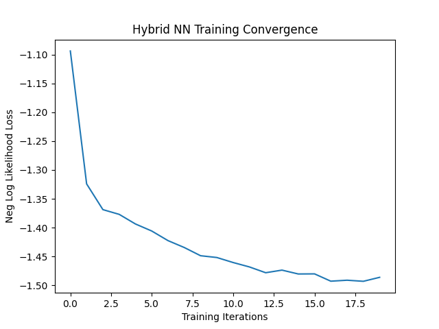
Let's also have a simple “plotting” electron to visualize how training progressed.

@ct.electron(executor=cpu_executor)
def plot_loss(epoch_loss):
    plt.plot(epoch_loss)
    plt.title("Hybrid NN Training Convergence")
    plt.xlabel("Training Iterations")
    plt.ylabel("Neg Log Likelihood Loss")
    plt.savefig('/tmp/plot.png')
    return Image.open('/tmp/plot.png')

Finally, the last electron will do model evaluations on unseen data to validate the model performance after training. We use the gpu_executor here as well, to access GPUs and speed up evaluation.

@ct.electron(executor=gpu_executor)
def evaluate(test_loader, model_path):
    import cudaq

    device = torch.device("cuda:0")

    kernel, thetas = cudaq.make_kernel(list)
    # load model
    model = Net(device, kernel, thetas).to(device)
    model.load_state_dict(torch.load(model_path))
    loss_func = nn.NLLLoss().to(device)

    model.eval()
    with torch.no_grad():
        correct = 0
        for batch_idx, (data, target) in enumerate(test_loader):
            data, target = data.to(device), target.to(device)
            output = model(data).to(device)

            pred = output.argmax(dim=1, keepdim=True)
            correct += pred.eq(target.view_as(pred)).sum().item()

            loss = loss_func(output, target)

        print(
            "Performance on test data:\n\tAccuracy: {:.1f}%".format(
                correct / len(test_loader) * 100
            )
        )
    return correct / len(test_loader) * 100

Workflow

To collect the above tasks (i.e. the electrons) into a workflow, we define a “main” function (called hybrid_cudaq_workflow here) and decorate it with @ct.lattice.

@ct.lattice(workflow_executor=cpu_executor, executor=cpu_executor)
def hybrid_cudaq_workflow(
    train_sample_count=140,
    test_sample_count=70,
    learning_rates=[0.001],  # hyperparameter list to loop over
    epochs=[20]              # here as well
):
    train_loader, test_loader = get_data(train_sample_count, test_sample_count)
    plots, accuracies = [], []
    for learning_rate in learning_rates:
        for epoch in epochs:
            model, epoch_loss = train_model(train_loader, learning_rate, epoch)
            accuracy = evaluate(test_loader, model)
            plot = plot_loss(epoch_loss)
            plots.append((learning_rate, epoch, plot))
            accuracies.append((learning_rate, epoch, accuracy))

    return plots, accuracies

The workflow may then be executed by dispatching to Covalent Cloud and later fetching the result.

# Run the workflow across (2 learning rates) x (2 epoch numbers) = 4 trials.
dispatch_id = cc.dispatch(hybrid_cudaq_workflow, volume=volume)(
    train_sample_count=100, learning_rates=[0.001, 0.05], epochs=[5, 20]
)

# This bit can be run at any time, provided the dispatch_id is known.
plots, accuracies = cc.get_result(dispatch_id, wait=True).result.load()

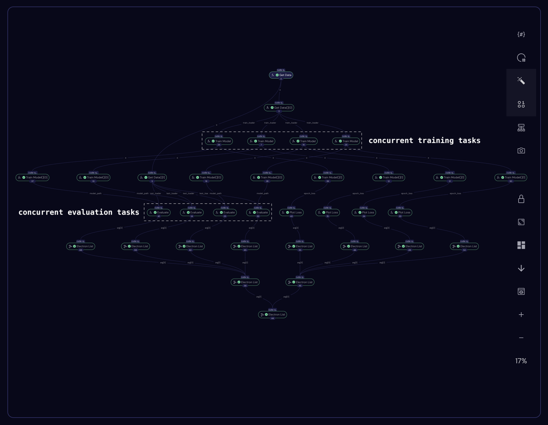
This workflow produces the following graph in the Covalent Cloud UI.

To inspect results, we can show returned loss plots in a Jupyter notebook by running e.g.

plots[1][-1]  # -> PIL.PngImagePlugin.PngImageFile object

Conclusion

In this tutorial, we combined Covalent Cloud, CUDA Quantum, and PyTorch to train and evaluate a hybrid quantum neural network. We also discussed choosing between CPU and GPU executors, and how to store data with Covalent Cloud volumes. If you execute the provided workflow using gpu_type='l40', the total cost will be ~$0.60.

The full code can be found below.

Full Code

# requirements:
# covalent-cloud>=0.81.0
# matplotlib==3.9.2
# numpy==1.23.5
# pillow==11.0.0
# torch==2.4.1
# torchvision==0.19.1

import covalent as ct
import covalent_cloud as cc

import matplotlib.pyplot as plt
import numpy as np
import torch
import torch.nn as nn
import torch.nn.functional as F
import torch.optim as optim
from PIL import Image
from torch.autograd import Function
from torchvision import datasets, transforms


cc.save_api_key("YOUR-API-KEY")  # NOTE: Replace with your real API key
cc.create_env(
    name="cuda-quantum",
    pip=[
        "cuda-quantum==0.8.0",
        "matplotlib==3.9.1",
        "torch==2.4.1",
        "torchvision==0.19.1",
    ],
    wait=True
)

volume = cc.volume("cudaq")

cpu_executor = cc.CloudExecutor(
    env="cuda-quantum",
    num_cpus=4,
    memory="16GB",
    time_limit=60*60  # 1 hour
)

gpu_executor = cc.CloudExecutor(
    env="cuda-quantum",
    num_gpus=1,
    gpu_type="h100",
    num_cpus=4,
    memory="16GB",
    time_limit=60*60
)


class QuantumFunction(Function):

    def __init__(self, qubit_count: int, device, kernel, thetas):
        """Define the quantum circuit in CUDA Quantum"""
        self.kernel = kernel
        self.theta = thetas
        self.device = device
        qubits = kernel.qalloc(qubit_count)
        self.kernel.h(qubits)
        # Variational gate parameters which are optimised during training.
        kernel.ry(thetas[0], qubits[0])
        kernel.rx(thetas[1], qubits[0])

    def run(self, thetas: torch.tensor) -> torch.tensor:
        """Execute the quantum circuit to output an expectation value"""
        import cudaq

        exp_ = cudaq.observe(self.kernel, cudaq.spin.z(0), thetas.tolist()).expectation()
        expectation = torch.tensor(exp_, device=self.device)
        return expectation

    @staticmethod
    def forward(ctx, thetas: torch.tensor, quantum_circuit, shift) -> torch.tensor:

        # Save shift and quantum_circuit in context to use in backward.
        ctx.shift = shift
        ctx.quantum_circuit = quantum_circuit

        # Calculate expectation value.
        expectation = ctx.quantum_circuit.run(thetas)

        ctx.save_for_backward(thetas, expectation)
        return expectation

    @staticmethod
    def backward(ctx, grad_output):
        """Backward pass computation via finite difference parameter shift"""
        thetas, expectation = ctx.saved_tensors

        device = ctx.quantum_circuit.device

        gradients = torch.zeros(len(thetas), device=device)
        for i in range(len(thetas)):
            shift_right = torch.clone(thetas)
            shift_right[i] += ctx.shift
            shift_left = torch.clone(thetas)
            shift_left[i] -= ctx.shift

            expectation_right = ctx.quantum_circuit.run(shift_right)
            expectation_left = ctx.quantum_circuit.run(shift_left)
            gradients[i] = (expectation_right -
                            expectation_left) / 2 * ctx.shift
        return gradients * grad_output.float(), None, None


class QuantumLayer(nn.Module):
    """Encapsulates a quantum circuit and a quantum function into a quantum layer"""

    def __init__(
        self, qubit_count: int, shift: torch.tensor, device, kernel, thetas
    ):
        super(QuantumLayer, self).__init__()

        self.device = device
        # 1 qubit quantum circuit.
        self.quantum_circuit = QuantumFunction(
            qubit_count, device, kernel, thetas
        )
        self.shift = shift

    def forward(self, input):
        ans = QuantumFunction.apply(input, self.quantum_circuit, self.shift)
        return ans


class Net(nn.Module):

    def __init__(self, device, kernel, thetas, qubit_count=1, shift=torch.tensor(np.pi / 2)):
        super(Net, self).__init__()

        # Neural network structure.
        self.conv1 = nn.Conv2d(1, 6, kernel_size=5)
        self.conv2 = nn.Conv2d(6, 16, kernel_size=5)
        self.dropout = nn.Dropout2d()
        self.fc1 = nn.Linear(256, 64)
        self.fc2 = nn.Linear(
            64, 2
        )  # Output a 2D tensor since we have 2 variational parameters in our quantum circuit.
        self.hybrid = QuantumLayer(
            qubit_count, shift, device, kernel, thetas
        )  # Input is the magnitude of the parameter shifts to calculate gradients.

    def forward(self, x):
        x = F.relu(self.conv1(x))
        x = F.max_pool2d(x, 2)
        x = F.relu(self.conv2(x))
        x = F.max_pool2d(x, 2)
        x = self.dropout(x)
        x = x.view(1, -1)
        x = F.relu(self.fc1(x))
        # Reshapes required to satisfy input dimensions to CUDA Quantum.
        x = self.fc2(x).reshape(-1)
        x = self.hybrid(x).reshape(-1)
        return torch.cat((x, 1 - x), -1).unsqueeze(0)


@ct.electron(executor=cpu_executor)
def get_data(train_sample_count, test_sample_count):
    data_path = volume / "data"
    X_train = datasets.MNIST(
        root=data_path,
        train=True,
        download=True,
        transform=transforms.Compose([transforms.ToTensor()]),
    )
    # Leaving only labels 0 and 1.
    idx = np.append(
        np.where(X_train.targets == 0)[0][:train_sample_count],
        np.where(X_train.targets == 1)[0][:train_sample_count],
    )
    X_train.data = X_train.data[idx]
    X_train.targets = X_train.targets[idx]
    train_loader = torch.utils.data.DataLoader(X_train, batch_size=1, shuffle=True)

    X_test = datasets.MNIST(
        root=data_path,
        train=False,
        download=True,
        transform=transforms.Compose([transforms.ToTensor()]),
    )
    idx = np.append(
        np.where(X_test.targets == 0)[0][:test_sample_count],
        np.where(X_test.targets == 1)[0][:test_sample_count],
    )
    X_test.data = X_test.data[idx]
    X_test.targets = X_test.targets[idx]
    test_loader = torch.utils.data.DataLoader(X_test, batch_size=1, shuffle=True)

    return train_loader, test_loader


@ct.electron(executor=gpu_executor)
def train_model(train_loader, learning_rate, epochs):
    import cudaq

    device = torch.device("cuda:0" if torch.cuda.is_available() else "cpu")

    kernel, thetas = cudaq.make_kernel(list)
    model = Net(device, kernel, thetas).to(device)
    optimizer = optim.Adam(model.parameters(), lr=learning_rate)
    loss_func = nn.NLLLoss().to(device)

    epochs = epochs
    epoch_loss = []
    model.train()

    for epoch in range(epochs):
        batch_loss = 0.0
        for batch_idx, (data, target) in enumerate(train_loader):  # Batch training.
            optimizer.zero_grad()
            data, target = data.to(device), target.to(device)

            # Forward pass.
            output = model(data).to(device)
            # Calculating loss.
            loss = loss_func(output, target).to(device)

            # Backward pass.
            loss.backward()

            # Optimize the weights.
            optimizer.step()
            batch_loss += loss.item()

        epoch_loss.append(batch_loss / batch_idx)

        print("Training [{:.0f}%]\tLoss: {:.4f}".format(100.0 * (epoch + 1) / epochs, epoch_loss[-1]))

    # save model
    model_path = volume / "model.pth"
    torch.save(model.state_dict(), model_path)

    return model_path, epoch_loss


@ct.electron(executor=cpu_executor)
def plot_loss(epoch_loss):
    plt.plot(epoch_loss)
    plt.title("Hybrid NN Training Convergence")
    plt.xlabel("Training Iterations")
    plt.ylabel("Neg Log Likelihood Loss")
    plt.savefig('/tmp/plot.png')
    return Image.open('/tmp/plot.png')


@ct.electron(executor=gpu_executor)
def evaluate(test_loader, model_path):
    import cudaq

    device = torch.device("cuda:0" if torch.cuda.is_available() else "cpu")

    kernel, thetas = cudaq.make_kernel(list)
    # load model
    model = Net(device, kernel, thetas).to(device)
    model.load_state_dict(torch.load(model_path))
    loss_func = nn.NLLLoss().to(device)

    model.eval()
    with torch.no_grad():
        correct = 0
        for batch_idx, (data, target) in enumerate(test_loader):
            data, target = data.to(device), target.to(device)
            output = model(data).to(device)

            pred = output.argmax(dim=1, keepdim=True)
            correct += pred.eq(target.view_as(pred)).sum().item()

            loss = loss_func(output, target)

        print(
            "Performance on test data:\n\tAccuracy: {:.1f}%".format(
                correct / len(test_loader) * 100
            )
        )
    return correct / len(test_loader) * 100


@ct.lattice(workflow_executor=cpu_executor, executor=cpu_executor)
def hybrid_cudaq_workflow(
    train_sample_count=140,
    test_sample_count=70,
    learning_rates=[0.001],  # hyperparameter list to loop over
    epochs=[20]              # here as well
):
    train_loader, test_loader = get_data(train_sample_count, test_sample_count)
    plots, accuracies = [], []
    for learning_rate in learning_rates:
        for epoch in epochs:
            model, epoch_loss = train_model(train_loader, learning_rate, epoch)
            accuracy = evaluate(test_loader, model)
            plot = plot_loss(epoch_loss)
            plots.append((learning_rate, epoch, plot))
            accuracies.append((learning_rate, epoch, accuracy))

    return plots, accuracies


if __name__ == "__main__":
    # Run the workflow across (2 learning rates) x (2 epoch numbers) = 4 trials.
    dispatch_id = cc.dispatch(hybrid_cudaq_workflow, volume=volume)(
        train_sample_count=100, learning_rates=[0.001, 0.05], epochs=[5, 20]
    )

    # This bit can be run at any time, provided the dispatch_id is known.
    plots, accuracies = cc.get_result(dispatch_id, wait=True).result.load()
    plots[1][-1].save("./plot_1.png")