GPU-accelerated quantum circuit simulations on Covalent Cloud

Quantum support-vector machines (QSVMs) are essentially traditional SVMs that rely on embedding kernels evaluated on a quantum computer—also known as a quantum embedding kernel. These kernels provide a unique (and perhaps classically-intractable) means of measuring pairwise similarity. Using GPUs to simulate quantum computers is worthwhile when qubit capacity and/or fidelity requirements are not met by the available quantum hardware. While QSVMs are relatively tolerant to noise (an important reason for their current popularity), evaluating kernels on real quantum hardware is not always practical nor necessary.

In this tutorial, we’ll demonstrate how to run GPU-accelerated quantum circuit simulations on Covalent Cloud.

Let’s start by importing the required packages.

import covalent as ct
import covalent_cloud as cc
import matplotlib.pyplot as plt
import pennylane as qml
from matplotlib.colors import ListedColormap
from pennylane import numpy as np
from sklearn.datasets import make_blobs
from sklearn.inspection import DecisionBoundaryDisplay
from sklearn.model_selection import train_test_split
from sklearn.svm import SVC

cc.save_api_key("API_KEY")

Covalent Cloud allows us to create re-usable execution environments, as shown below. This environment represents a typical setup for running Pennylane on NVIDIA GPUs.

cc.create_env(
    name="pennylane-gpu",  # identifier for referring to this environment
    conda={
        "channels": ["conda-forge"],
        "dependencies": ["cudatoolkit>=11.8"],
    }, pip=[
        "cuquantum==23.10.0",
        "matplotlib==3.8.2",
        "Pennylane==0.34.0",
        "PennyLane-Lightning[GPU]==0.34.0",
        "scikit-learn==1.3.1",
        "torch==2.1.2",
    ],
    wait=True
)

Next, we'll define our resource specifications by creating some executors for this workflow. Both executors will run tasks in our new environment, named ”pennylane-gpu”.

cpu_executor = cc.CloudExecutor(  # for lightweight non-quantum tasks
    env="pennylane-gpu",
    num_cpus=1,
    memory="1GB",
)
gpu_executor = cc.CloudExecutor(  # for GPU-powered circuit simulations
    env="pennylane-gpu",
    num_cpus=4,
    memory="12GB",
    num_gpus=1,
    gpu_type="v100"
)

On to the algorithm!

Here's a function returns a simple quantum kernel based on Pennylane's IQP Embedding template. We'll use it as-is inside our workflow.

QML_DEVICE = "lightning.gpu"

def get_kernel_circuit(n_wires):

    @qml.qnode(qml.device(QML_DEVICE, wires=n_wires, shots=None))
    def circuit(x1, x2):
        qml.IQPEmbedding(x1, wires=range(n_wires), n_repeats=4)
        qml.adjoint(qml.IQPEmbedding)(x2, wires=range(n_wires), n_repeats=4)
        return qml.probs(wires=range(n_wires))

    return lambda x1, x2: circuit(x1, x2)[0]  # |0..0> state probability

Next, each function destined for remote execution is decorated with @ct.electron, with an executor specified therein. Only tasks that evaluate the simulated quantum kernel should require gpu_executor. For example, we don't need GPUs to generate our input data:

@ct.electron(executor=cpu_executor)  # lightweight non-quantum task
def get_split_data(n_samples=18, test_size=0.2):
    centers = [(1, 1), (1, 2), (1, 3), (2, 1), (2, 2), (2, 3), (3, 1), (3, 2), (3, 3)]
    X, y = make_blobs(n_samples, centers=centers, cluster_std=0.25, shuffle=False)
    # rescale labels to be -1, 1
    mapping = {0: -1, 1: 1, 2: -1, 3: 1, 4: -1, 5: 1, 6: -1, 7: 1, 8: -1}
    y = np.array([mapping[i] for i in y])
    X = X.astype(np.float32)
    y = y.astype(int)

    # X_train, X_test, y_train, y_test
    return train_test_split(X, y, test_size=test_size, random_state=3)

Classifying with the SVM, on the other hand, requires $O(n^2)$ kernel evaluations, where $n$ is the dataset size. Accordingly, we'll use GPUs (i.e. gpu_executor) to speed up this process.

DISP_SETTINGS = {"grid_resolution": 50, "response_method": "predict", "alpha": 0.5, "cmap": plt.cm.RdBu}

@ct.electron(executor=gpu_executor)
def classify_with_qsvm(Xtr, Xte, ytr, yte):
    kernel = get_kernel_circuit(n_wires=Xtr.shape[1])

    kernel_matrix_fn = lambda X, Z: qml.kernels.kernel_matrix(X, Z, kernel)
    svc = SVC(kernel=kernel_matrix_fn).fit(Xtr, ytr)

    # train/test accuracy
    accuracy_tr = svc.score(Xtr, ytr)
    accuracy_te = svc.score(Xte, yte)

    # decision boundary
    cm_bright = ListedColormap(["#FF0000", "#0000FF"])
    disp = DecisionBoundaryDisplay.from_estimator(svc, Xte, **DISP_SETTINGS)
    disp.ax_.scatter(Xtr[:, 0], Xtr[:, 1], c=ytr, cmap=cm_bright)
    disp.ax_.scatter(Xte[:, 0], Xte[:, 1], c=yte, cmap=cm_bright, marker="$\u25EF$")

    return accuracy_tr, accuracy_te, disp

Putting it all together, we can define a QSVM training and testing workflow. This special function gets decorated with @ct.lattice.

@ct.lattice(workflow_executor=cpu_executor, executor=cpu_executor)
def run_qsvm(n_samples, test_size):
    Xtr, Xte, ytr, yte = get_split_data(n_samples, test_size)
    return classify_with_qsvm(Xtr, Xte, ytr, yte)

Now, to dispatch run_qsvm to Covalent Cloud, we call it after wrapping with ct.dispatch, as usual.

dispatch_id = cc.dispatch(run_qsvm)(n_samples=36, test_size=0.2)
print("Dispatch ID:", dispatch_id)

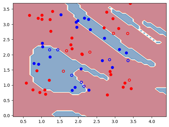
Here's what we get when we query and display the results.

result = cc.get_result(dispatch_id, wait=True)
result.result.load()

train_acc, test_acc, decision_boundary_figure = result.result.value
print(f"Train accuracy: {train_acc * 100:.1f}%")
print(f"Test accuracy: {test_acc * 100:.1f}%")

decision_boundary_figure  # show in notebook

Output:

Train accuracy: 80.4%
Test accuracy: 69.2%

Conclusion

In this tutorial, we demonstrated how to run quantum circuit simulations on GPUs via Covalent Cloud. We used Pennylane to define a simple quantum kernel, and then trained and tested a QSVM on a 2-dimensional dataset. To make the most of this tutorial, try experimenting with different datasets/kernels or increasing the dataset dimension, to gain a greater advantage from GPU acceleration.

The cost of running this workflow is approximately $0.27. The full code is available below.

Full code

import covalent as ct
import covalent_cloud as cc
import matplotlib.pyplot as plt
import pennylane as qml
from matplotlib.colors import ListedColormap
from pennylane import numpy as np
from sklearn.datasets import make_blobs
from sklearn.inspection import DecisionBoundaryDisplay
from sklearn.model_selection import train_test_split
from sklearn.svm import SVC

cc.save_api_key("API_KEY")

cc.create_env(
    name="pennylane-gpu",  # identifier for referring to this environment
    conda={
        "channels": ["conda-forge"],
        "dependencies": ["cudatoolkit>=11.8"],
    }, pip=[
        "cuquantum==23.10.0",
        "matplotlib==3.8.2",
        "Pennylane==0.34.0",
        "PennyLane-Lightning[GPU]==0.34.0",
        "scikit-learn==1.3.1",
        "torch==2.1.2",
    ],
    wait=True
)

cpu_executor = cc.CloudExecutor(  # for lightweight non-quantum tasks
    env="pennylane-gpu",
    num_cpus=2,
    memory="2GB",
)
gpu_executor = cc.CloudExecutor(  # for GPU-powered circuit simulations
    env="pennylane-gpu",
    num_cpus=4,
    memory="12GB",
    num_gpus=1,
    gpu_type="v100"
)

QML_DEVICE = "lightning.gpu"

def get_kernel_circuit(n_wires):

    @qml.qnode(qml.device(QML_DEVICE, wires=n_wires, shots=None))
    def circuit(x1, x2):
        qml.IQPEmbedding(x1, wires=range(n_wires), n_repeats=4)
        qml.adjoint(qml.IQPEmbedding)(x2, wires=range(n_wires), n_repeats=4)
        return qml.probs(wires=range(n_wires))

    return lambda x1, x2: circuit(x1, x2)[0]  # |0..0> state probability

@ct.electron(executor=cpu_executor)  # lightweight non-quantum task
def get_split_data(n_samples=18, test_size=0.2):
    centers = [(1, 1), (1, 2), (1, 3), (2, 1), (2, 2), (2, 3), (3, 1), (3, 2), (3, 3)]
    X, y = make_blobs(n_samples, centers=centers, cluster_std=0.25, shuffle=False)
    # rescale labels to be -1, 1
    mapping = {0: -1, 1: 1, 2: -1, 3: 1, 4: -1, 5: 1, 6: -1, 7: 1, 8: -1}
    y = np.array([mapping[i] for i in y])
    X = X.astype(np.float32)
    y = y.astype(int)

    # X_train, X_test, y_train, y_test
    return train_test_split(X, y, test_size=test_size, random_state=3)

DISP_SETTINGS = {"grid_resolution": 50, "response_method": "predict", "alpha": 0.5, "cmap": plt.cm.RdBu}

@ct.electron(executor=gpu_executor)
def classify_with_qsvm(Xtr, Xte, ytr, yte):
    kernel = get_kernel_circuit(n_wires=Xtr.shape[1])

    kernel_matrix_fn = lambda X, Z: qml.kernels.kernel_matrix(X, Z, kernel)
    svc = SVC(kernel=kernel_matrix_fn).fit(Xtr, ytr)

    # train/test accuracy
    accuracy_tr = svc.score(Xtr, ytr)
    accuracy_te = svc.score(Xte, yte)

    # decision boundary
    cm_bright = ListedColormap(["#FF0000", "#0000FF"])
    disp = DecisionBoundaryDisplay.from_estimator(svc, Xte, **DISP_SETTINGS)
    disp.ax_.scatter(Xtr[:, 0], Xtr[:, 1], c=ytr, cmap=cm_bright)
    disp.ax_.scatter(Xte[:, 0], Xte[:, 1], c=yte, cmap=cm_bright, marker="$\u25EF$")

    return accuracy_tr, accuracy_te, disp

@ct.lattice(workflow_executor=cpu_executor, executor=cpu_executor)
def run_qsvm(n_samples, test_size):
    Xtr, Xte, ytr, yte = get_split_data(n_samples, test_size)
    return classify_with_qsvm(Xtr, Xte, ytr, yte)

dispatch_id = cc.dispatch(run_qsvm)(n_samples=64, test_size=0.2)
print("Dispatch ID:", dispatch_id)

result = cc.get_result(dispatch_id, wait=True)
result.result.load()

train_acc, test_acc, decision_boundary_figure = result.result.value
print(f"Train accuracy: {train_acc * 100:.1f}%")
print(f"Test accuracy: {test_acc * 100:.1f}%")