Violating the CHSH Inequality on IBM Quantum Backends

Background

The CHSH inequality is an important result related to Bell’s theorem, which shows that quantum mechanics is incompatible with local hidden-variable theories. This means that there are results in quantum mechanics (see the Einstein-Podolsky-Rosen paradox) which cannot be explained by some unknown parameters that are local to the system being observed.

There are simple experiments on quantum computers that can show violation of the CHSH inequality. These experiments involve running computations on systems of entangled qubits. With Covalent QElectrons and free access to IBM Quantum backends, we can easily do this.

The CHSH Inequality

Physical systems that are compatible with local hidden variables must obey the following inequality.

$$|\langle S_{\mp} \rangle| = |\langle AB \rangle \mp \langle Ab \rangle \pm \langle aB \rangle + \langle ab \rangle| \leq 2 \qquad (1)$$

Here, $\langle \, \cdot \, \rangle$ refers to the expectation value of some observable. The value $\langle AB \rangle$, for example, is the average outcome of an experiment involving an $A$-basis measurement on the first qubit and a $B$-basis measurement on the second.

Testing the CHSH inequality requires two different measurement bases for each qubit, or four two-qubit measurement bases for the entire system. In our experiment, we take $b$ and $B$ to be the Pauli $Z$ and $X$ bases, while $a$ and $A$ taken to be the bases $Z^\prime$ and $X^\prime$. Crucially, the latter two are rotated (in the same plane) by some angle $\theta$ relative to $Z$ and $X$.

Experimental Demonstration of Bell’s Theorem

Our goal here will be to verify that the CHSH inequality $(1)$ is violated by a quantum system of two entangled qubits.

Procedure

This will involve the following steps:

1. Prepare the two-qubit system in a Bell state.
2. Apply $Y$-rotation by an angle $\theta$ to the first qubit only.
3. Measure the system in the $ZZ$, $ZX$, $XZ$, or $XX$ basis.
4. Repeat steps 1-3 many times to estimate the expectation value.
5. Repeat steps 1-4 to obtain estimates for all four bases which are used to compute $\langle S_{\mp} \rangle$.

Note that $Y$-rotating the first qubit before measurement is equivalent here to measuring that qubit in a rotated basis. Therefore, the expectation values we obtain are indeed the $\langle Z^\prime Z \rangle$, $\langle Z^\prime X \rangle$, $\langle X^\prime Z \rangle$, and $\langle X^\prime X \rangle$ required to compute $|\langle S_{\mp} \rangle|$.

Quantum Circuit

The circuit we need is one that prepares a Bell state:

$$|\Phi^{+}\rangle = \frac{1}{\sqrt{2}}(|00\rangle + |11\rangle)$$

Briefly, the state $|\Phi^{+}\rangle$ is said to be “maximally entangled” because measuring either qubit will determine the measurement outcome of the other with perfect accuracy (when both qubits are measured in the same basis). This is easy to verify by looking at the basis states that make up $|\Phi^{+}\rangle$.

State preparation is straightforward. Starting with the $|00\rangle$ state, applying a Hadamard on the first qubit, followed by a CNOT gate produces $|\Phi^{+}\rangle$. We also apply an additional $Y$-rotation of the first qubit by $\theta$ to control offset between the respective measurements.

import pennylane as qml

observables = [
    qml.PauliZ(0) @ qml.PauliZ(1),
    qml.PauliZ(0) @ qml.PauliX(1),
    qml.PauliX(0) @ qml.PauliZ(1),
    qml.PauliX(0) @ qml.PauliX(1),
]

dev = qml.device("default.qubit", wires=2, shots=8192)

@qml.qnode(dev)
def chsh_circuit(theta):
    # Prepare Bell state.
    qml.Hadamard(wires=0)
    qml.CNOT(wires=[0, 1])

    # Apply Y-rotation by angle `theta`.
    qml.RY(theta, wires=0)

    # Multiple returns to get all 4 expectation values.
    return [qml.expval(obs) for obs in observables]

Creating QElectrons

With the code above, we can easily perform a simulated version of this experiment using regular Pennylane. To make for a more interesting experiment, we can use Covalent QElectrons to try this on various IBM QPUs.

For example, a QElectron that runs on "ibmq_lima" is defined below.

# Define a quantum executor that targets the "ibmq_lima" QPU.
ibmq_lima = ct.executor.QiskitExecutor(
    device="sampler",
    backend="ibmq_lima",
    single_job=True,
        ibmqx_token="<token>"
)

# Create a QElectron from the Pennylane QNode.
# qcircuit_lima = ct.qelectron(chsh_circuit, executors=ibmq_lima)

When making a QiskitExecutor, users can additionally pass the keyword arguments

• hub
• group
• project

to take advantage of privileged IBM Quantum access by their organization. The executor’s ibmqx_token argument can be omitted if provided in the Covalent configuration file (typically at ~/.config/covalent/covalent.conf). We shall assume that this is the case for brevity going forward.

Below we define a few more quantum executors for later use.

# NOTE: assume `ibmqx_token` provided in Covalent configuration.

# Define a quantum executor that targets "ibm_lagos" QPU.
ibm_lagos = ct.executor.QiskitExecutor(
    device="sampler",
    backend="ibm_lagos",
    single_job=True,
)

# Define quantum executors for two IBM simulators.
ibmq_qasm_simulator = ct.executor.QiskitExecutor(
        device="sampler",
        backend="ibmq_qasm_simulator",
)

simulator_statevector = ct.executor.QiskitExecutor(
        device="sampler",
        backend="simulator_statevector",
)

Covalent Workflow

Let’s use these executors in a Covalent workflow that tests the CHSH inequality. To briefly outline the workflow, we have

• a task that runs the experiment on "ibmq_lima"
• a task that runs the experiment on "ibm_lagos"
• a task that uses both "ibmq_qasm_simulator" and "simulator_statevector" as a Quantum Cluster, distributing circuits evenly between the two.

Finally, the compute_S_mp() task uses the estimated expectation values to calculate $\langle S_{\mp} \rangle$ for all three cases.

import covalent as ct
from pennylane import numpy as np


@ct.electron
def get_thetas():
    """Generates a range of angles `theta`."""
    return np.linspace(0, 2 * np.pi, 25)


@ct.electron
def chsh_on_lima(thetas):
    """Runs the angle sweep on 'ibmq_lima' QPU."""
    qelectron = ct.qelectron(chsh_circuit, executors=ibmq_lima)
    expvals_list = qelectron(thetas)
    return np.asarray(expvals_list)


@ct.electron
def chsh_on_lagos(thetas):
    """Runs the angle sweep on 'ibm_lagos' QPU."""
    qelectron = ct.qelectron(chsh_circuit, executors=ibm_lagos)
    expvals_list = qelectron(thetas)
    return np.asarray(expvals_list)


@ct.electron
def chsh_on_simulators(thetas):
    """
    Uses a cluster of of two simulators to run the angle sweep.
    """
    executors = [ibmq_qasm_simulator, simulator_statevector]
    qelectron = ct.qelectron(chsh_circuit, executors=executors)
    expvals_list = qelectron(thetas)
    return np.asarray(expvals_list)


@ct.electron
def compute_S_mp(expvals: dict):
    """Computes S_mins and S_plus from Equation (1)."""
    results = {}
    for name, expvals_arr in expvals.items():

        AB, Ab, aB, ab = expvals_arr
        S_minus = AB - Ab + aB + ab
        S_plus = AB + Ab - aB + ab
        results[name] = (S_minus, S_plus)

    return results


@ct.lattice
def workflow():

    thetas = get_thetas()
    expvals = {}

    # QPU experiments.
    expvals["lima"] = chsh_on_lima(thetas)
    expvals["lagos"] = chsh_on_lagos(thetas)

    # Simulator experiment.
    expvals["simulators"] = chsh_on_simulators(thetas)

    # Evaluate the CHSH inequality.
    results = compute_S_mp(expvals)

    return thetas, expvals, results

Running the following will dispatch the workflow and wait for the results.

dispatch_id = ct.dispatch(workflow)()
print(dispatch_id)
thetas, expvals, results = ct.get_result(dispatch_id, wait=True).result

Looking at the Covalent UI, we can see that the simulator experiments completed in ~1 minute. The QPU experiments (chsh_on_lagos() and chsh_on_lima()) can take much longer depending on the queue times for the two devices. In our workflow, Covalent mitigates this at the task level, with both tasks queueing for QPUs at the same time.

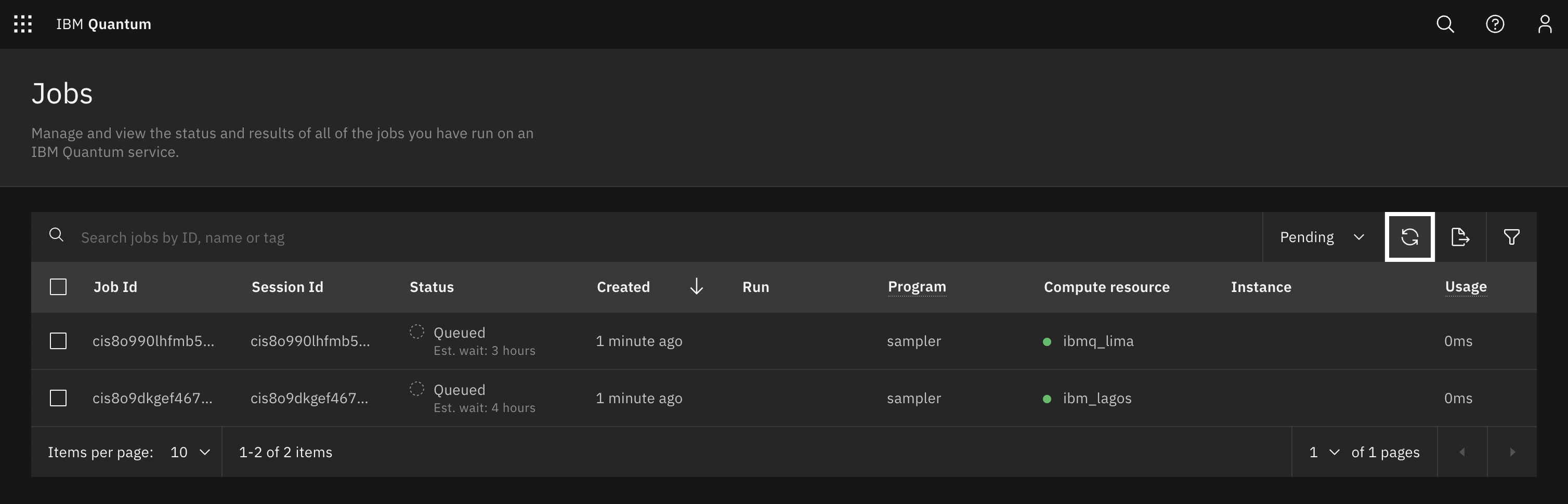
IBM Quantum queue showing “ibmq_lima” and “ibm_lagos” jobs queued simultaneously.

Covalent workflow showing the completed simulator task and pending QPU tasks.

Note that there is additionally circuit-level parallelism provided by QElectrons themselves. In this workflow, chsh_on_simulators() uses a cluster of simulators and distributes individual circuit calls across two different backends.

Altogether, the experiment completed in about 40 minutes.

Analysis

The workflow results are plotted below, using a function given in the Appendix.

Four curves inhabit each subplot. The dashed and dotted grey lines represent $\langle S_{-} \rangle$ and $\langle S_{+} \rangle$ from the cluster of simulators. These curves are shown on both subplots for comparison. The orange and purples lines represent $\langle S_{-} \rangle$ and $\langle S_{+} \rangle$ for "ibmq_lima" on the left, and similarly for "ibm_lagos" on the right.

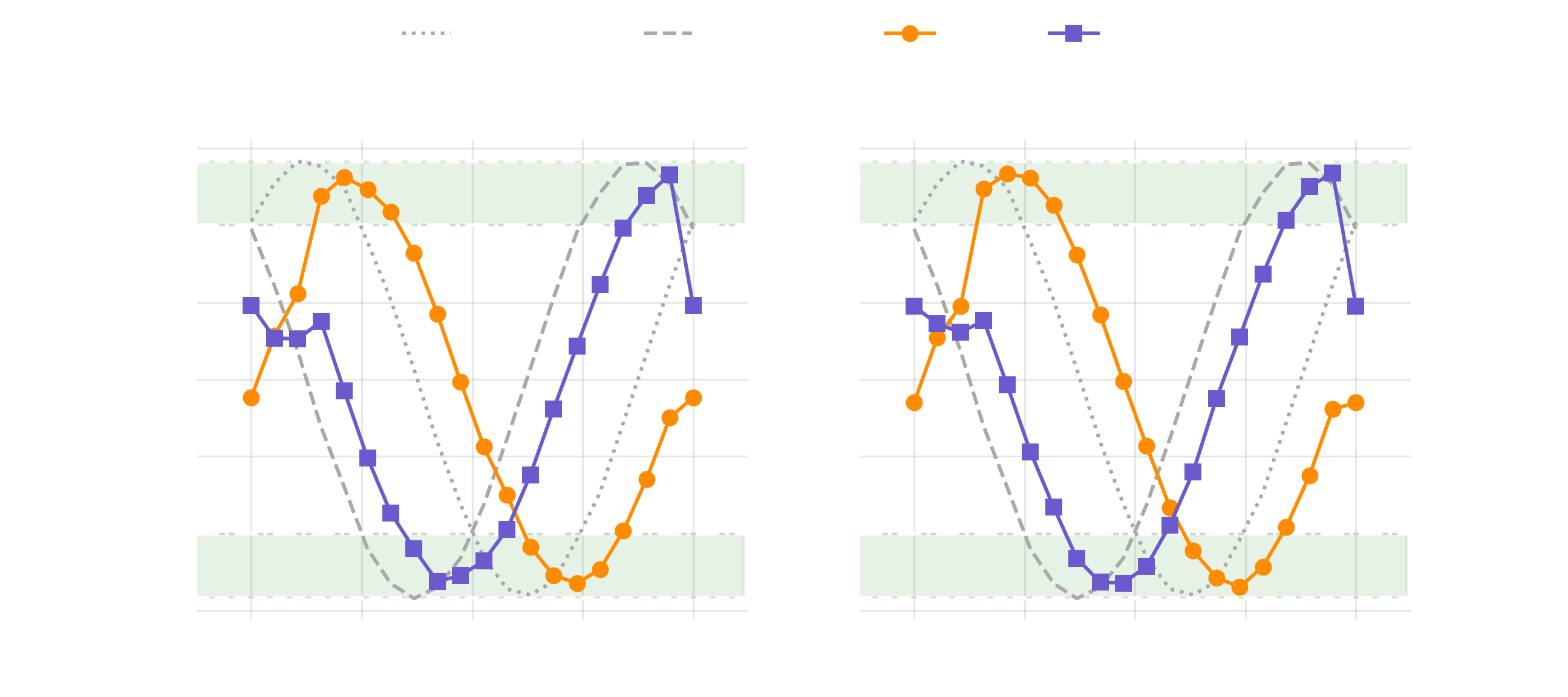
It’s easiest to see from the simulated (sim.) results that either the $|\langle S_{-} \rangle|$ or $|\langle S_{+} \rangle|$ is always greater than $2$ for all $\theta$ between $0$ and $2\pi$. In other words, the CHSH inequality is violated for any non-trivial rotation between the pairs of bases.

This is not so obvious from the hardware results, where noise at large and small $\theta$ somewhat obscures the intended outcome. Interesting to note, there is also significant phase error in the hardware results—and this is quite convenient for our plot.

This tutorial is based on the Qiskit Runtime example found here.