Comparing Deep Learning Models for Sales Forecasting using Covalent

Summary

In this example, we use Covalent to orchestrate a workflow which compares the performances of four different deep learning models -- the multi-layer perceptron (MLP) model, the convolutional neural network (CNN) model, the long short-term memory (LSTM) model, and a hybrid CNN-LSTM model. Each neural network is trained on daily historical sales data spanning four years. Covalent allows us to easily deploy different tasks to different hardware resources.

About Covalent

The Covalent API is a Python module containing a small collection of classes that implement server-based workflow management. The key elements are two decorators that wrap functions to create managed tasks and workflows.

The task decorator is called an electron. The @electron decorator simply turns the function into a dispatchable task. The workflow decorator is called a lattice. The @lattice decorator turns a function composed of electrons into a manageable workflow.

Covalent Features Used

In order to transform our data and train our models we will be leveraging AWS resources to offload those tasks to remote machines with our desired amount of compute resources. Below are all of the features of covalent that we use for this tutorial.

• To upload our dataset to an S3 bucket we will utilize Covalent's FileTransfer functionallity
• In order for covalent to be able to execute tasks in a remote environment we will need to declare which pip packages are to be installed for specific tasks using DepsPip
• We will be offloading the dataset transformation tasks to AWS ECS using the AWS ECS Executor
• Finally we will be training the models in an AWS Batch compute environment using the AWS Batch Executor

Heterogeneity

Tasks in this example are heterogeneous in several ways:

• Task Scheduling: Dask / AWS ECS (Fargate) / AWS Batch
• Execution Backend: Local / Remote CPU

Overview of Tutorial

The workflow performs the following steps:

Task	Resources
1. Fetch and validate a training dataset from a remote machine
2. Explore the dataset and visualize broad trends
3. Clean / transform the data
4. Split the Data for Training and Validation
5. Construct the DNN Models
6. Train the Models
7. Visualize the results

This tutorial is derived from work by Dimitre Oliveira on Kaggle.

In order for the workflow to succeed with the corresponding dataset, it's important to assign 2 GB of memory to each of the workers. For this workflow, Covalent was started with:

covalent start -n 4 -m "2GB"

Implementation

Fetch and validate a training dataset from a remote machine

We first import all of the libraries that are intended to be used

with open("./requirements.txt", "r") as file:
    for line in file:
        print(line.rstrip())

covalent
pandas==1.4.4
tensorflow==2.9.1

# Install required packages
# !pip install -r ./requirements.txt

# Imports
import covalent as ct

import cloudpickle
import warnings
import numpy as np
import pandas as pd
from tensorflow.keras import optimizers
from keras.utils.vis_utils import plot_model
from keras.models import Sequential, Model
from keras.layers.convolutional import Conv1D, MaxPooling1D
from keras.layers import Dense, LSTM, RepeatVector, TimeDistributed, Flatten
from sklearn.metrics import mean_squared_error
from sklearn.model_selection import train_test_split
import plotly.graph_objs as go
from plotly.offline import init_notebook_mode, iplot
from typing import List

import matplotlib
import matplotlib.pyplot as plt

matplotlib.use("Agg")

warnings.filterwarnings("ignore")
init_notebook_mode(connected=True)

from tensorflow.random import set_seed
from numpy.random import seed

set_seed(1)
seed(1)

from covalent._shared_files import logger

app_log = logger.app_log

We construct the first task, which fetches input data from a remote machine

data_bucket_uri = "s3://dnn-tutorial-dataset"
strategy = ct.fs_strategies.S3(
    credentials="/home/user/.aws/credentials", profile="default", region_name="us-east-1"
)


@ct.electron(
    files=[
        ct.fs.TransferFromRemote(
            f"{data_bucket_uri}/train.csv", order=ct.fs.Order.BEFORE, strategy=strategy
        ),
        ct.fs.TransferFromRemote(
            f"{data_bucket_uri}/test.csv", order=ct.fs.Order.BEFORE, strategy=strategy
        ),
    ]
)
def fetch_and_validate_data(files=[]) -> List[str]:
    _, local_train = files[0]
    _, local_test = files[1]
    train = pd.read_csv(local_train, parse_dates=["date"])
    test = pd.read_csv(local_test, parse_dates=["date"])
    return train, test

Explore the dataset and visualize broad trends

Next, explore the dataset and visualize basic trends

@ct.electron
def explore_data(dataset):
    # Aggregate daily sales
    daily_sales = dataset.groupby("date", as_index=False)["sales"].sum()
    store_daily_sales = dataset.groupby(["store", "date"], as_index=False)["sales"].sum()
    item_daily_sales = dataset.groupby(["item", "date"], as_index=False)["sales"].sum()

    # Plot total daily sales
    daily_sales_sc = go.Scatter(x=daily_sales["date"], y=daily_sales["sales"])
    layout1 = go.Layout(title="Daily sales", xaxis=dict(title="Date"), yaxis=dict(title="Sales"))
    fig1 = go.Figure(data=[daily_sales_sc], layout=layout1)

    # Sales by item
    item_daily_sales_sc = []
    for item in item_daily_sales["item"].unique():
        current_item_daily_sales = item_daily_sales[(item_daily_sales["item"] == item)]
        item_daily_sales_sc.append(
            go.Scatter(
                x=current_item_daily_sales["date"],
                y=current_item_daily_sales["sales"],
                name=("Item %s" % item),
            )
        )

    layout2 = go.Layout(
        title="Item daily sales", xaxis=dict(title="Date"), yaxis=dict(title="Sales")
    )
    fig2 = go.Figure(data=item_daily_sales_sc, layout=layout2)

    return fig1, fig2

Clean / transform the data

Now we subsample and transform the data to a period of interest. We use the last year of data and for each date, use the previous month to forecast 90 days ahead. In addition, this task will run on AWS Fargate on ECS.

In order to run this electron on a remote executor, we need to specify the package dependcies via ct.DepsPip(...).

ecs_executor = ct.executor.ECSExecutor(
    credentials="/home/user/.aws/credentials",
    region="us-east-1",
    profile="default",
    ecr_repo_name="dnn-tutorial-ecs-ecr-repo",
    ecs_cluster_name="dnn-tutorial-ecs-ecs-cluster",
    ecs_task_execution_role_name="dnn-tutorial-ecs-task-execution-role",
    ecs_task_log_group_name="dnn-tutorial-ecs-log-group",
    ecs_task_role_name="dnn-tutorial-ecs-task-role",
    ecs_task_security_group_id="sg-03f5c620fa4d4d5fc",
    ecs_task_subnet_id="subnet-0127aa9a0344152d0",
    s3_bucket_name="dnn-tutorial-ecs-bucket",
    vcpu=4,
    memory=8,
    retry_attempts=2,
    poll_freq=10,
    time_limit=3000,
    cache_dir="/tmp/covalent",
)

deps_pip = ct.DepsPip(packages=["pandas==1.4.4"])


@ct.electron(
    deps_pip=deps_pip,
    executor=ecs_executor,
    files=[
        ct.fs.TransferFromRemote(
            f"{data_bucket_uri}/train.csv", order=ct.fs.Order.BEFORE, strategy=strategy
        ),
        ct.fs.TransferToRemote(
            f"{data_bucket_uri}/time_series.csv", order=ct.fs.Order.AFTER, strategy=strategy
        ),
    ],
)
def transform_data(window, lag_size, files=[]):
    _, local_train = files[0]
    dataset = pd.read_csv(local_train)

    # Subsample
    refined_data = dataset[(dataset["date"] >= "2017-01-01")]

    # Restructure
    group = refined_data.sort_values("date").groupby(["item", "store", "date"], as_index=False)
    group = group.agg({"sales": ["mean"]})
    group.columns = ["item", "store", "date", "sales"]

    data = group.drop("date", axis=1)
    cols, names = list(), list()

    # Input sequence (t-n, ... t-1)
    for i in range(window, 0, -1):
        cols.append(data.shift(i))
        names += [("%s(t-%d)" % (col, i)) for col in data.columns]

    # Current timestep (t=0)
    cols.append(data)
    names += [("%s(t)" % (col)) for col in data.columns]

    # Target timestep (t=lag)
    cols.append(data.shift(-lag_size))
    names += [("%s(t+%d)" % (col, lag_size)) for col in data.columns]

    # Put it all together
    time_series = pd.concat(cols, axis=1)
    time_series.columns = names

    # Drop rows with NaN values
    time_series.dropna(inplace=True)

    # Filter unwanted data
    last_item = "item(t-%d)" % window
    last_store = "store(t-%d)" % window
    time_series = time_series[(time_series["store(t)"] == time_series[last_store])]
    time_series = time_series[(time_series["item(t)"] == time_series[last_item])]

    columns_to_drop = [("%s(t+%d)" % (col, lag_size)) for col in ["item", "store"]]
    for i in range(window, 0, -1):
        columns_to_drop += [("%s(t-%d)" % (col, i)) for col in ["item", "store"]]
    time_series.drop(columns_to_drop, axis=1, inplace=True)
    time_series.drop(["item(t)", "store(t)"], axis=1, inplace=True)

    app_log.debug(f"Transformed size info: {time_series.shape}")

    from_file, to_file = files[1]
    time_series.to_csv(from_file, index=False)

Split the Data for Training and Validation

We store the data in the s3 bucket since they can potentially be very large and we want to avoid unnecessary pickling and unpickling during the workflow execution.

# Split the time series into training / validation sets
@ct.electron(
    files=[
        ct.fs.TransferFromRemote(
            f"{data_bucket_uri}/time_series.csv", order=ct.fs.Order.BEFORE, strategy=strategy
        ),
        ct.fs.TransferToRemote(
            f"{data_bucket_uri}/X_train.pkl", order=ct.fs.Order.AFTER, strategy=strategy
        ),
        ct.fs.TransferToRemote(
            f"{data_bucket_uri}/X_train_series.pkl", order=ct.fs.Order.AFTER, strategy=strategy
        ),
        ct.fs.TransferToRemote(
            f"{data_bucket_uri}/X_valid.pkl", order=ct.fs.Order.AFTER, strategy=strategy
        ),
        ct.fs.TransferToRemote(
            f"{data_bucket_uri}/X_valid_series.pkl", order=ct.fs.Order.AFTER, strategy=strategy
        ),
        ct.fs.TransferToRemote(
            f"{data_bucket_uri}/Y_train.pkl", order=ct.fs.Order.AFTER, strategy=strategy
        ),
        ct.fs.TransferToRemote(
            f"{data_bucket_uri}/Y_valid.pkl", order=ct.fs.Order.AFTER, strategy=strategy
        ),
    ]
)
def split_data(lag_size, files=[]):
    # Read file from s3 bucket
    to_file, from_file = files[0]
    time_series = pd.read_csv(from_file)

    # Label
    labels_col = "sales(t+%d)" % lag_size
    labels = time_series[labels_col]
    time_series = time_series.drop(labels_col, axis=1)

    X_train, X_valid, Y_train, Y_valid = train_test_split(
        time_series, labels.values, test_size=0.4, random_state=0
    )
    X_train_series = X_train.values.reshape((X_train.shape[0], X_train.shape[1], 1))
    X_valid_series = X_valid.values.reshape((X_valid.shape[0], X_valid.shape[1], 1))

    for idx, obj in enumerate(
        [X_train, X_train_series, X_valid, X_valid_series, Y_train, Y_valid]
    ):
        from_file, to_file = files[idx + 1]
        with open(from_file, "wb") as f:
            cloudpickle.dump(obj, f)

Construct the DNN Models

Next frame contruction of the four DNN models as tasks.

@ct.electron(
    files=[
        ct.fs.TransferFromRemote(
            f"{data_bucket_uri}/X_train.pkl", order=ct.fs.Order.BEFORE, strategy=strategy
        ),
    ]
)
def construct_mlp_model(files=[]):
    from_file, to_file = files[0]
    with open(to_file, "rb") as f:
        X_train = cloudpickle.load(f)
    model_mlp = Sequential()
    model_mlp.add(Dense(100, activation="relu", input_dim=X_train.shape[1]))
    model_mlp.add(Dense(1))

    return model_mlp

@ct.electron(
    files=[
        ct.fs.TransferFromRemote(
            f"{data_bucket_uri}/X_train_series.pkl", order=ct.fs.Order.BEFORE, strategy=strategy
        ),
    ]
)
def construct_cnn_model(files=[]):
    with open(files[0][1], "rb") as f:
        X_train_series = cloudpickle.load(f)

    model_cnn = Sequential()
    model_cnn.add(
        Conv1D(
            filters=64,
            kernel_size=2,
            activation="relu",
            input_shape=(X_train_series.shape[1], X_train_series.shape[2]),
        )
    )
    model_cnn.add(MaxPooling1D(pool_size=2))
    model_cnn.add(Flatten())
    model_cnn.add(Dense(50, activation="relu"))
    model_cnn.add(Dense(1))

    return model_cnn

@ct.electron(
    files=[
        ct.fs.TransferFromRemote(
            f"{data_bucket_uri}/X_train_series.pkl", order=ct.fs.Order.BEFORE, strategy=strategy
        ),
    ]
)
def construct_lstm_model(files=[]):
    with open(files[0][1], "rb") as f:
        X_train_series = cloudpickle.load(f)

    model_lstm = Sequential()
    model_lstm.add(
        LSTM(50, activation="relu", input_shape=(X_train_series.shape[1], X_train_series.shape[2]))
    )
    model_lstm.add(Dense(1))

    return model_lstm

@ct.electron(
    files=[
        ct.fs.TransferFromRemote(
            f"{data_bucket_uri}/X_train_series.pkl", order=ct.fs.Order.BEFORE, strategy=strategy
        ),
        ct.fs.TransferFromRemote(
            f"{data_bucket_uri}/X_valid_series.pkl", order=ct.fs.Order.BEFORE, strategy=strategy
        ),
    ]
)
def construct_cnn_lstm_model(files=[]):
    with open(files[0][1], "rb") as f:
        X_train_series = cloudpickle.load(f)

    with open(files[1][1], "rb") as f:
        X_valid_series = cloudpickle.load(f)

    subsequences = 2
    timesteps = X_train_series.shape[1] // subsequences
    app_log.debug(
        f"Tensor shape info: {(X_train_series.shape[0], X_train_series.shape[1], timesteps)}"
    )
    X_train_series_sub = X_train_series.reshape(
        (X_train_series.shape[0], subsequences, timesteps, 1)
    )
    X_valid_series_sub = X_valid_series.reshape(
        (X_valid_series.shape[0], subsequences, timesteps, 1)
    )

    model_cnn_lstm = Sequential()
    model_cnn_lstm.add(
        TimeDistributed(
            Conv1D(filters=64, kernel_size=1, activation="relu"),
            input_shape=(None, X_train_series_sub.shape[2], X_train_series_sub.shape[3]),
        )
    )
    model_cnn_lstm.add(TimeDistributed(MaxPooling1D(pool_size=2)))
    model_cnn_lstm.add(TimeDistributed(Flatten()))
    model_cnn_lstm.add(LSTM(50, activation="relu"))
    model_cnn_lstm.add(Dense(1))

    return model_cnn_lstm

Train the Models

Define tasks which train / fit the four models. We will offload these to a remote AWS Batch backend.

batch_executor = ct.executor.AWSBatchExecutor(
    credentials="/home/user/.aws/credentials",
    profile="default",
    batch_execution_role_name="dnn-tutorial-batch-task-execution-role",
    batch_job_definition_name="dnn-tutorial-batch-job-definition",
    batch_job_log_group_name="dnn-tutorial-batch-log-group",
    batch_job_role_name="dnn-tutorial-batch-job-role",
    batch_queue="dnn-tutorial-batch-queue",
    s3_bucket_name="dnn-tutorial-batch-job-resources",
    vcpu=2,
    memory=4,
    retry_attempts=2,
    poll_freq=10,
    time_limit=3000,
    cache_dir="/tmp/covalent",
)

deps_pip = ct.DepsPip(packages=["tensorflow==2.9.1", "pandas==1.4.4", "cloudpickle==2.0.0"])


@ct.electron(
    deps_pip=deps_pip,
    executor=batch_executor,
    files=[
        ct.fs.TransferFromRemote(
            f"{data_bucket_uri}/X_train.pkl", order=ct.fs.Order.AFTER, strategy=strategy
        ),
        ct.fs.TransferFromRemote(
            f"{data_bucket_uri}/X_valid.pkl", order=ct.fs.Order.AFTER, strategy=strategy
        ),
        ct.fs.TransferFromRemote(
            f"{data_bucket_uri}/Y_train.pkl", order=ct.fs.Order.AFTER, strategy=strategy
        ),
        ct.fs.TransferFromRemote(
            f"{data_bucket_uri}/Y_valid.pkl", order=ct.fs.Order.AFTER, strategy=strategy
        ),
    ],
)
def fit_mlp_model(model_mlp, learning_rate, epochs, files=[]):
    with open(files[0][1], "rb") as f:
        X_train = cloudpickle.load(f)

    with open(files[1][1], "rb") as f:
        X_valid = cloudpickle.load(f)

    with open(files[2][1], "rb") as f:
        Y_train = cloudpickle.load(f)

    with open(files[3][1], "rb") as f:
        Y_valid = cloudpickle.load(f)

    model_mlp.compile(loss="mse", optimizer=optimizers.Adam(learning_rate))

    return model_mlp.fit(
        X_train.values, Y_train, validation_data=(X_valid.values, Y_valid), epochs=epochs
    )

@ct.electron(
    deps_pip=deps_pip,
    executor=batch_executor,
    files=[
        ct.fs.TransferFromRemote(
            f"{data_bucket_uri}/X_train_series.pkl", order=ct.fs.Order.AFTER, strategy=strategy
        ),
        ct.fs.TransferFromRemote(
            f"{data_bucket_uri}/X_valid_series.pkl", order=ct.fs.Order.AFTER, strategy=strategy
        ),
        ct.fs.TransferFromRemote(
            f"{data_bucket_uri}/Y_train.pkl", order=ct.fs.Order.AFTER, strategy=strategy
        ),
        ct.fs.TransferFromRemote(
            f"{data_bucket_uri}/Y_valid.pkl", order=ct.fs.Order.AFTER, strategy=strategy
        ),
    ],
)
def fit_cnn_model(model_cnn, learning_rate, epochs, files=[]):
    with open(files[0][1], "rb") as f:
        X_train_series = cloudpickle.load(f)

    with open(files[1][1], "rb") as f:
        X_valid_series = cloudpickle.load(f)

    with open(files[2][1], "rb") as f:
        Y_train = cloudpickle.load(f)

    with open(files[3][1], "rb") as f:
        Y_valid = cloudpickle.load(f)

    model_cnn.compile(loss="mse", optimizer=optimizers.Adam(learning_rate))

    return model_cnn.fit(
        X_train_series, Y_train, validation_data=(X_valid_series, Y_valid), epochs=epochs
    )

@ct.electron(
    deps_pip=deps_pip,
    executor=batch_executor,
    files=[
        ct.fs.TransferFromRemote(
            f"{data_bucket_uri}/X_train_series.pkl", order=ct.fs.Order.AFTER, strategy=strategy
        ),
        ct.fs.TransferFromRemote(
            f"{data_bucket_uri}/X_valid_series.pkl", order=ct.fs.Order.AFTER, strategy=strategy
        ),
        ct.fs.TransferFromRemote(
            f"{data_bucket_uri}/Y_train.pkl", order=ct.fs.Order.AFTER, strategy=strategy
        ),
        ct.fs.TransferFromRemote(
            f"{data_bucket_uri}/Y_valid.pkl", order=ct.fs.Order.AFTER, strategy=strategy
        ),
    ],
)
def fit_lstm_model(model_lstm, learning_rate, epochs, files=[]):
    with open(files[0][1], "rb") as f:
        X_train_series = cloudpickle.load(f)

    with open(files[1][1], "rb") as f:
        X_valid_series = cloudpickle.load(f)

    with open(files[2][1], "rb") as f:
        Y_train = cloudpickle.load(f)

    with open(files[3][1], "rb") as f:
        Y_valid = cloudpickle.load(f)

    model_lstm.compile(loss="mse", optimizer=optimizers.Adam(learning_rate))

    return model_lstm.fit(
        X_train_series, Y_train, validation_data=(X_valid_series, Y_valid), epochs=epochs
    )

@ct.electron(
    deps_pip=deps_pip,
    executor=batch_executor,
    files=[
        ct.fs.TransferFromRemote(
            f"{data_bucket_uri}/X_train_series.pkl", order=ct.fs.Order.AFTER, strategy=strategy
        ),
        ct.fs.TransferFromRemote(
            f"{data_bucket_uri}/X_valid_series.pkl", order=ct.fs.Order.AFTER, strategy=strategy
        ),
        ct.fs.TransferFromRemote(
            f"{data_bucket_uri}/Y_train.pkl", order=ct.fs.Order.AFTER, strategy=strategy
        ),
        ct.fs.TransferFromRemote(
            f"{data_bucket_uri}/Y_valid.pkl", order=ct.fs.Order.AFTER, strategy=strategy
        ),
    ],
)
def fit_cnn_lstm_model(model_cnn_lstm, learning_rate, epochs, files=[]):
    with open(files[0][1], "rb") as f:
        X_train_series = cloudpickle.load(f)

    with open(files[1][1], "rb") as f:
        X_valid_series = cloudpickle.load(f)

    with open(files[2][1], "rb") as f:
        Y_train = cloudpickle.load(f)

    with open(files[3][1], "rb") as f:
        Y_valid = cloudpickle.load(f)

    model_cnn_lstm.compile(loss="mse", optimizer=optimizers.Adam(learning_rate))

    subsequences = 2
    timesteps = X_train_series.shape[1] // subsequences
    X_train_series_sub = X_train_series.reshape(
        (X_train_series.shape[0], subsequences, timesteps, 1)
    )
    X_valid_series_sub = X_valid_series.reshape(
        (X_valid_series.shape[0], subsequences, timesteps, 1)
    )

    return model_cnn_lstm.fit(
        X_train_series_sub, Y_train, validation_data=(X_valid_series_sub, Y_valid), epochs=epochs
    )

Visualize the results

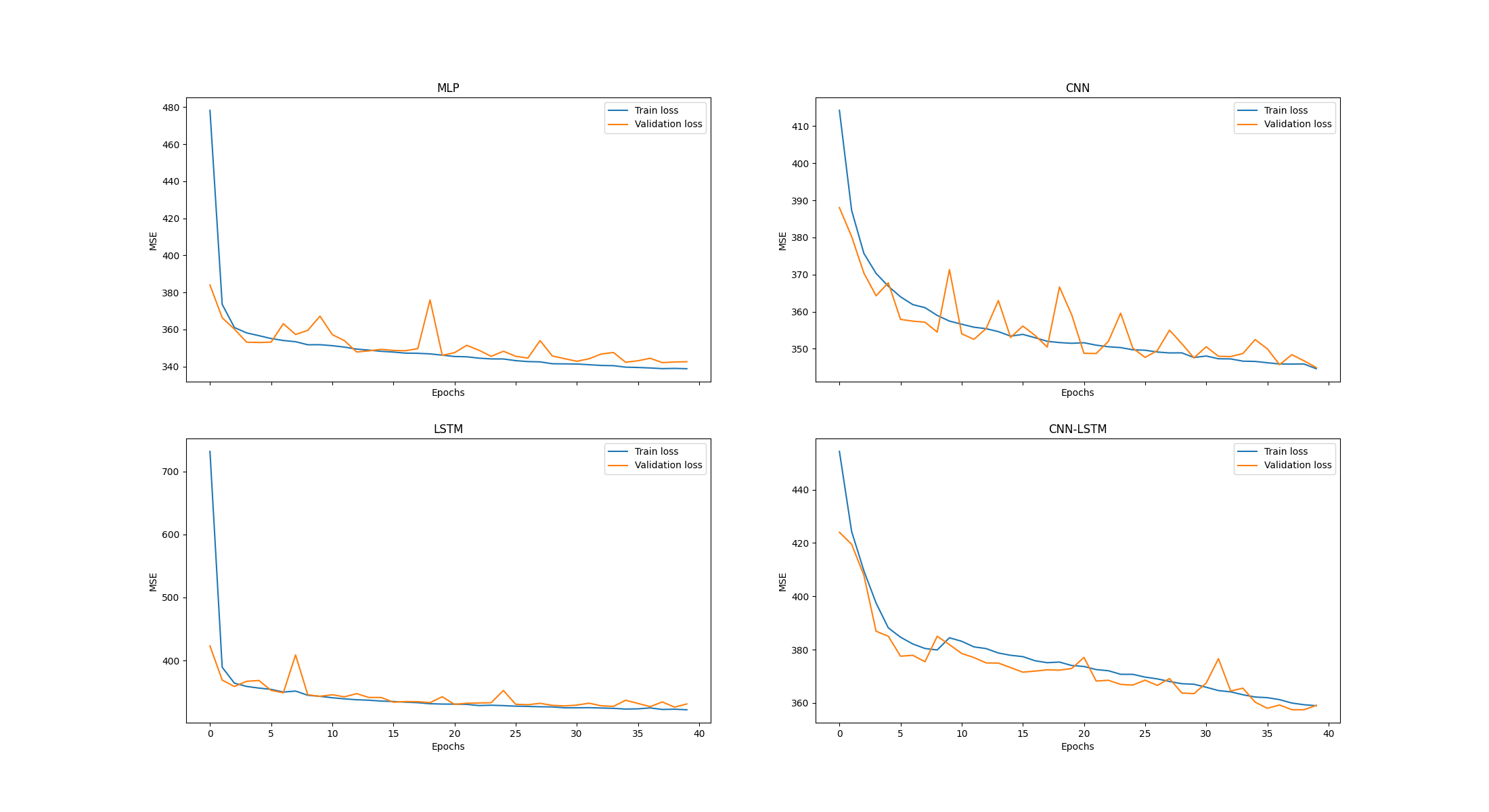
We then plot our loss fuctions with respect to epochs

@ct.electron
def visualize_loss_functions(mlp_history, cnn_history, lstm_history, cnn_lstm_history):
    fig, axes = plt.subplots(2, 2, sharex=True, sharey=False, figsize=(22,12))
    ax1, ax2 = axes[0]
    ax3, ax4 = axes[1]

    ax1.plot(mlp_history.history['loss'], label='Train loss')
    ax1.plot(mlp_history.history['val_loss'], label='Validation loss')
    ax1.legend(loc='best')
    ax1.set_title('MLP')
    ax1.set_xlabel('Epochs')
    ax1.set_ylabel('MSE')

    ax2.plot(cnn_history.history['loss'], label='Train loss')
    ax2.plot(cnn_history.history['val_loss'], label='Validation loss')
    ax2.legend(loc='best')
    ax2.set_title('CNN')
    ax2.set_xlabel('Epochs')
    ax2.set_ylabel('MSE')

    ax3.plot(lstm_history.history['loss'], label='Train loss')
    ax3.plot(lstm_history.history['val_loss'], label='Validation loss')
    ax3.legend(loc='best')
    ax3.set_title('LSTM')
    ax3.set_xlabel('Epochs')
    ax3.set_ylabel('MSE')

    ax4.plot(cnn_lstm_history.history['loss'], label='Train loss')
    ax4.plot(cnn_lstm_history.history['val_loss'], label='Validation loss')
    ax4.legend(loc='best')
    ax4.set_title('CNN-LSTM')
    ax4.set_xlabel('Epochs')
    ax4.set_ylabel('MSE')
    plt.savefig("/tmp/comparison.png")

Compare Models

We are now ready to construct a workflow which compares four DNN models using a variety of cloud-based compute resources

@ct.lattice
def compare_models(window, lag_size, learning_rate, epochs):
    # Fetch and validate source data
    train, test = fetch_and_validate_data()

    # Explore the data
    daily_sales_plt, sales_by_item_plt = explore_data(train)

    # Subsample and transform the data followed by splitting the dataset
    transform_data_call = transform_data(window, lag_size)
    split_data_call = split_data(lag_size)

    ct.wait(child=split_data_call, parents=[transform_data_call])

    # Construct the models
    model_mlp = construct_mlp_model()
    ct.wait(child=model_mlp, parents=[split_data_call])

    model_cnn = construct_cnn_model()
    ct.wait(child=model_cnn, parents=[split_data_call])

    model_lstm = construct_lstm_model()
    ct.wait(child=model_lstm, parents=[split_data_call])

    model_cnn_lstm = construct_cnn_lstm_model()
    ct.wait(child=model_cnn_lstm, parents=[split_data_call])

    # Train the models
    mlp_history = fit_mlp_model(model_mlp=model_mlp, learning_rate=learning_rate, epochs=epochs)
    ct.wait(child=mlp_history, parents=[model_mlp])

    cnn_history = fit_cnn_model(model_cnn=model_cnn, learning_rate=learning_rate, epochs=epochs)
    ct.wait(child=cnn_history, parents=[model_cnn])

    lstm_history = fit_lstm_model(
        model_lstm=model_lstm, learning_rate=learning_rate, epochs=epochs
    )
    ct.wait(child=lstm_history, parents=[model_lstm])

    cnn_lstm_history = fit_cnn_lstm_model(
        model_cnn_lstm=model_cnn_lstm, learning_rate=learning_rate, epochs=epochs
    )
    ct.wait(child=cnn_lstm_history, parents=[model_cnn_lstm])

    # Generate loss function plot
    visualize_loss_functions(mlp_history, cnn_history, lstm_history, cnn_lstm_history)

    return mlp_history, cnn_history, lstm_history, cnn_lstm_history

Run the workflow!

dispatch_id = ct.dispatch(compare_models)(window=29, lag_size=90, learning_rate=0.0003, epochs=40)

print(dispatch_id)

1eeb141a-518c-4f9b-8aaf-10d46beca7de

Last Steps

You are now free to kill the Python kernel, take a walk, and come back when your workflow is done running. Want reminders? Ask about e-mail or Slack notifications upon completion/failure...

But first, let's now take a look at the UI in the browser...

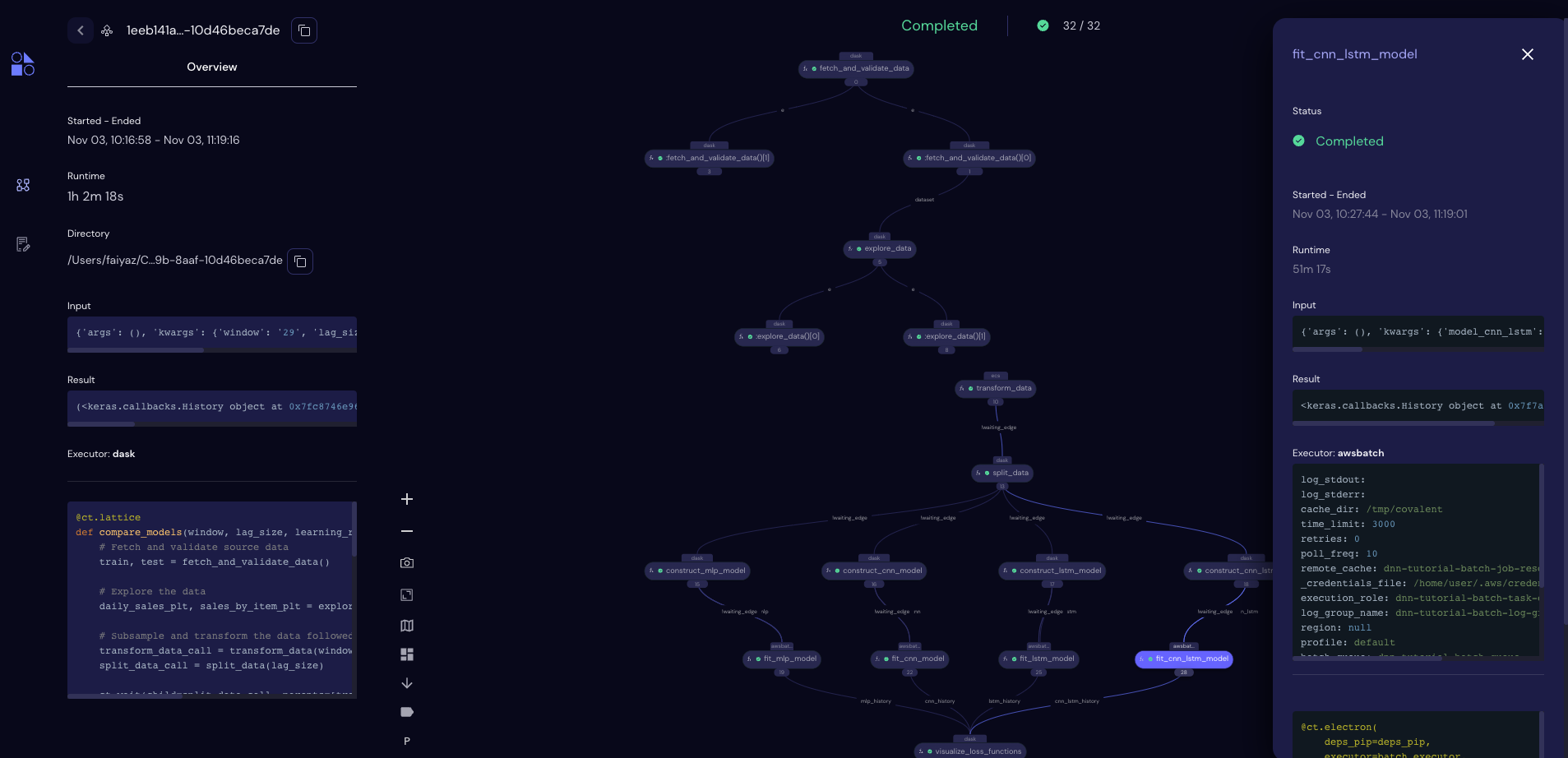
res = ct.get_result(dispatch_id, wait=True)

print(
    f"Workflow status: {res.status} \nComputation time: {((res.end_time - res.start_time).total_seconds() / 60):.1f} minutes"
)

Workflow status: COMPLETED
Computation time: 62.3 minutes

Plots

Finally, let's visualize the loss functions for each of the models as they trained